Advection; Resolution Test (2D)
This example presents a grid-resolution test for the two-dimensional advection schemes. The numerical setup is identical to that used in the 2D advection example.
To evaluate the accuracy and resolution dependence of each advection scheme, the script calculates the following diagnostic quantities:
- the relative deviation of the final maximum temperature from its initial value,
- the final maximum temperature, and
- the final spatial mean temperature.
The first diagnostic measures the magnitude of the change in the maximum temperature during advection. A decrease generally reflects numerical diffusion, whereas an increase may indicate numerical overshooting or interpolation errors. With increasing grid resolution, the diagnostic quantities should approach their corresponding reference values.
First one needs to load the required packages:
using Plots, Interpolations, Statistics
using GeoModBox.AdvectionEquation.TwoD
using GeoModBox.InitialCondition, GeoModBox.Tracers.TwoD
using Base.Threads
using Printf, TimerOutputs, LaTeXStrings, Measures
The following section defines the maximum resolution and the advection schemes to be tested. The maximum resolution is given by:
\[\begin{equation} n_{x,\max} = n_{\mathrm{res}}\,n_{x,0}, \end{equation}\]
where $n_{\mathrm{res}}$ is the number of tested resolution levels and $n_{x,0}=20$ is the resolution increment. The vertical resolution is set equal to the horizontal resolution, $n_y=n_x$.
@printf("Running on %d thread(s)\n", nthreads())

nrnxny      =   6
Scheme      =   ["upwind","slf","semilag","markers"]
ns          =   size(Scheme,1)
@show ns
save_fig    =   -1
The variable save_fig controls the plotting and file output:
save_fig = -1: save only the final summary figures;save_fig = 0: display the generated figures without saving animations;save_fig = 1: save the GIF animation for every scheme and resolution, as well as the final summary figures.
Generating all animations is computationally expensive and is therefore not recommended for large resolution tests.
Next, initialize the statistical parameters used for the resolution analysis.
# Statistical Parameter ============================================== #
St      = (
    Δ           =   zeros(size(Scheme,1),nrnxny),
    nxny        =   zeros(size(Scheme,1),nrnxny),
    Tmax        =   zeros(size(Scheme,1),nrnxny),
    Tmean       =   zeros(size(Scheme,1),nrnxny),
)
p3 = plot(layout=(2,2),
        dpi = 300, size=(1200,900))
panel   =   ["a)","b)","c)","d)"]
# -------------------------------------------------------------------- #
The next step defines the initial conditions, model geometry, and constants for visualization.
# Define Initial Condition =========================================== #
# Temperature ---
#   1) circle, 2) gaussian, 3) block
# Velocity ---
#   1) RigidBody, 2) ShearCell
Ini         =   (T=:circle,V=:RigidBody,)
# -------------------------------------------------------------------- #
# Model Constants ==================================================== #
M   =   (
    xmin    =   0.0,
    xmax    =   1.0,
    ymin    =   0.0,
    ymax    =   1.0,
)
BC  =   ()  # dummy
# -------------------------------------------------------------------- #
# Plot constants ===================================================== #
Pl  =   (
    inc         =   5,
    sc          =   1.0e9,
    Minc        =   1,
    Msz         =   0.2,
)
# -------------------------------------------------------------------- #
The simulation begins with a loop over the different advection schemes.
for m = 1:ns # Loop over advection schemes
    # Define Numerical Scheme ======================================== #
    FD          =   (Method     = (Adv=Scheme[m],),)
    @printf("Advection Scheme: %s\n ",string(FD.Method.Adv))
    # ---------------------------------------------------------------- #
For each scheme, a nested loop is used to iterate over different grid resolutions. Within the loop, one needs to update the grid resolution and coordinates.
    for l = 1:nrnxny # Loop over differnet resolutions
        # Numerical Constants ======================================== #
        NC  =   (
            x       =   l*20,       # Number of horizontal centroids
            y       =   l*20,       # Number of vertical centroids
        )
        display(string("nx = ",NC.x,", ny = ",NC.y))
        NV =   (
            x       =   NC.x + 1,   # Number of horizontal vertices
            y       =   NC.y + 1,   # Number of vertical vertices
        )
        Δ   =   (
            x   =   (abs(M.xmin)+M.xmax)/NC.x,
            y   =   (abs(M.ymin)+M.ymax)/NC.y,
        )
        # ------------------------------------------------------------ #
        # Grid ======================================================= #
        x   =   (
            c       =   LinRange(M.xmin + Δ.x/2.0, M.xmax - Δ.x/2.0, NC.x),
            ce      =   LinRange(M.xmin - Δ.x/2.0, M.xmax + Δ.x/2.0, NC.x+2),
            v       =   LinRange(M.xmin, M.xmax , NV.x)
        )
        y       = (
            c       =   LinRange(M.ymin + Δ.y/2.0, M.ymax - Δ.y/2.0, NC.y),
            ce      =   LinRange(M.ymin - Δ.y/2.0, M.ymax + Δ.y/2.0, NC.y+2),
            v       =   LinRange(M.ymin, M.ymax, NV.y),
        )
        x1      =   (
            c2d     =   x.c .+ 0*y.c',
            v2d     =   x.v .+ 0*y.v',
            vx2d    =   x.v .+ 0*y.ce',
            vy2d    =   x.ce .+ 0*y.v',
        )
        x   =   merge(x,x1)
        y1      =   (
            c2d     =   0*x.c .+ y.c',
            v2d     =   0*x.v .+ y.v',
            vx2d    =   0*x.v .+ y.ce',
            vy2d    =   0*x.ce .+ y.v',
        )
        y   =   merge(y,y1)
        # ------------------------------------------------------------ #
To enable visualization, the output path and filename for the animation are defined. In addition, memory is allocated for the required data fields.
        # Animationsettings ========================================== #
        path        =   string("./examples/AdvectionEquation/Results/")
        anim        =   Plots.Animation(path, String[] )
        filename    =   string("2D_advection_",Ini.T,"_",Ini.V,
                                "_",FD.Method.Adv,"_",NC.x,"_",NC.y,
                                "_nth_",nthreads())
        # ------------------------------------------------------------ #
        # Array Initialization ======================================= #
        D       =   (
            T       =   zeros(Float64,(NC.x,NC.y)),
            T_ex    =   zeros(Float64,(NC.x+2,NC.y+2)),
            T_exo   =   zeros(Float64,(NC.x+2,NC.y+2)),
            Told_ex =   zeros(Float64,(NC.x+2,NC.y+2)),
            vx      =   zeros(Float64,(NV.x,NV.y+1)),
            vy      =   zeros(Float64,(NV.x+1,NV.y)),
            vxc     =   zeros(Float64,(NC.x,NC.y)),
            vyc     =   zeros(Float64,(NC.x,NC.y)),
            vc      =   zeros(Float64,(NC.x,NC.y)),
            wt      =   zeros(Float64,(NC.x,NC.y)),
            wte     =   zeros(Float64,(NC.x+2,NC.y+2)),
            wtv     =   zeros(Float64,(NV...)),
            Tmax    =   [0.0],
            Tmin    =   [0.0],
        )
Now, one can calculate the initial conditions. Here, the built-in functions for the initial temperature and velocity conditions, IniTemperature!() and IniVelocity!(), respectively, are used. For more information please refer to the documentation. Following the velocity initialization, one can calculate the velocity on the centroids.
        # Initial Condition ========================================== #
        @timeit to "IniCondition" begin
        # Temperature ---
        IniTemperature!(Ini.T,M,NC,D,x,y)
        if FD.Method.Adv == "slf"
            D.T_exo    .=  D.T_ex
        end
        D.Tmax[1]   =   maximum(D.T_ex)
        D.Tmin[1]   =   minimum(D.T_ex)
        # D.Tmean[1]  =   (D.Tmax[1]+D.Tmin[1])/2
        # Velocity ---
        IniVelocity!(Ini.V,D,BC,NV,Δ,M,x,y)            # [ m/s ]
        # Get the velocity on the centroids ---
        @threads for i = 1:NC.x
            for j = 1:NC.y
                D.vxc[i,j]  = (D.vx[i,j+1] + D.vx[i+1,j+1])/2
                D.vyc[i,j]  = (D.vy[i+1,j] + D.vy[i+1,j+1])/2
            end
        end
        @. D.vc        = sqrt(D.vxc^2 + D.vyc^2)
        end
        # ------------------------------------------------------------ #
Now, one needs to define the time parameter. Here, the maximum time is set such that the anomaly completes one full revolution.
        # Time ======================================================= #
        T   =   (
            tmax    =   [0.0],
            Δfac    =   1.0,    # Courant time factor, i.e. dtfac*dt_courant
            Δ       =   [0.0],
        )
        T.tmax[1]   =   π*((M.xmax-M.xmin)-2*Δ.x)/maximum(D.vc)   # t = U/v [ s ]
        T.Δ[1]      =   T.Δfac * minimum((Δ.x,Δ.y)) /
                    (sqrt(maximum(abs.(D.vx))^2 + maximum(abs.(D.vy))^2))
        nt          =   ceil(Int,T.tmax[1]/T.Δ[1])
        # ------------------------------------------------------------ #
If tracer are used one needs to initialize them in the following. For more information please refer to the documentation.
        # Tracer Advection =========================================== #
        if FD.Method.Adv == "markers"
            @timeit to "TracerIni" begin
            # Tracer Initialization ---
            nmx,nmy     =   5,5
            noise       =   1
            nmark       =   nmx*nmy*NC.x*NC.y
            Aparam      =   :thermal
            MPC         =   (
                c       =   zeros(Float64,(NC.x,NC.y)),
                v       =   zeros(Float64,(NV.x,NV.y)),
                th      =   zeros(Float64,(nthreads(),NC.x,NC.y)),
                thv     =   zeros(Float64,(nthreads(),NV.x,NV.y)),
            )
            MAVG        = (
                PC_th   =   [similar(D.wte) for _ = 1:nthreads()],  # per thread
                PV_th   =   [similar(D.wtv) for _ = 1:nthreads()],   # per thread
                wte_th  =   [similar(D.wte) for _ = 1:nthreads()],  # per thread
                wtv_th  =   [similar(D.wtv) for _ = 1:nthreads()],  # per thread
            )
            Ma      =   IniTracer2D(Aparam,nmx,nmy,Δ,M,NC,noise,0,0)
            # RK4 weights ---
            rkw     =   1.0/6.0*[1.0 2.0 2.0 1.0]   # for averaging
            rkv     =   1.0/2.0*[1.0 1.0 2.0 2.0]   # for time stepping
            # Interpolate on centroids ---
            @threads for k = 1:nmark
                Ma.T[k] =   FromCtoM(D.T_ex, k, Ma, x, y, Δ, NC)
            end
            ΔT_grid     =   zeros(Float64,(NC.x+2,NC.y+2))
            # Count marker per cell ---
            CountMPC(Ma,nmark,MPC,M,x,y,Δ,NC,NV)
            end
        end
        # ------------------------------------------------------------ #
Let's visualize the initial condition first.
        # Visualize initial condition -------------------------------- #
        if FD.Method.Adv == "markers"
            p = heatmap(x.c,y.c,(D.T./D.Tmax)',color=:thermal,
                    aspect_ratio=:equal,xlims=(M.xmin, M.xmax),
                    ylims=(M.ymin, M.ymax),clims=(0.5, 1.0),
                    colorbar=true, size = (1200,600), dpi = 300,
                                        title= latexstring("\\mathrm{", string(FD.Method.Adv), "}"),
                    layout=(1,2),subplot=1)
            quiver!(p,x.c2d[1:Pl.inc:end,1:Pl.inc:end],
                    y.c2d[1:Pl.inc:end,1:Pl.inc:end],
                    quiver=(D.vxc[1:Pl.inc:end,1:Pl.inc:end].*Pl.sc,
                            D.vyc[1:Pl.inc:end,1:Pl.inc:end].*Pl.sc),
                    color="white",
                    layout=(1,2),subplot=1)
            heatmap!(p,x.c,y.c,MPC.c',color=:inferno,
                    aspect_ratio=:equal,
                    xlims=(M.xmin, M.xmax),
                    ylims=(M.ymin, M.ymax),
                    colorbar=true,clims=(0.0, 18.0),
                    layout=(1,2),subplot=2)
        else
            p = heatmap(x.c , y.c, (D.T./D.Tmax)',
                    color=:thermal, colorbar=true, aspect_ratio=:equal,
                    xlabel= L"x", ylabel= L"z",
                    title= latexstring("\\mathrm{", string(FD.Method.Adv), "}"),
                    xlims=(M.xmin, M.xmax),
                    ylims=(M.ymin, M.ymax),
                    clims=(0.5, 1.0),
                    size = (900,900), dpi = 300,
                    guidefontsize = 20, tickfontsize = 20,
                    right_margin = 10mm,
                    titlefontsize = 20,
                    )
            quiver!(p,x.c2d[1:Pl.inc:end,1:Pl.inc:end],y.c2d[1:Pl.inc:end,1:Pl.inc:end],
                    quiver=(D.vxc[1:Pl.inc:end,1:Pl.inc:end].*Pl.sc,
                            D.vyc[1:Pl.inc:end,1:Pl.inc:end].*Pl.sc),
                    color="white")
        end
        if save_fig == 1
            Plots.frame(anim)
        elseif save_fig == 0
            display(p)
        end
        # ------------------------------------------------------------ #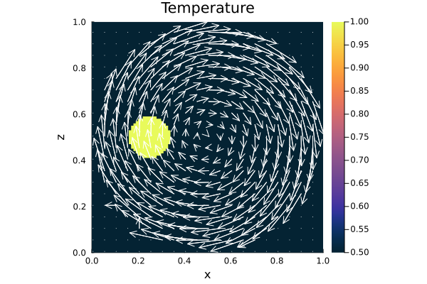
Figure 1. Initial condition. Initial rigid-body rotation setup with a circular temperature anomaly. The temperature is normalized by its initial maximum value, such that the maximum temperature equals one.
Now, one can start the time loop and the advection.
        # Time Loop ================================================== #
        for i = 2:nt
            if FD.Method.Adv == "upwind"
                upwindc2D!(D.T,D.T_ex,D.vxc,D.vyc,NC,T.Δ[1],Δ.x,Δ.y)
            elseif FD.Method.Adv == "slf"
                slfc2D!(D.T,D.T_ex,D.T_exo,D.vxc,D.vyc,NC,T.Δ[1],Δ.x,Δ.y)
            elseif FD.Method.Adv == "semilag"
                semilagc2D!(D.T,D.T_ex,D.vxc,D.vyc,D.vxc,D.vyc,x,y,T.Δ[1])
            elseif FD.Method.Adv == "markers"
                @. ΔT_grid     =   D.T_ex - D.Told_ex
                @threads for k = 1:nmark
                    local ΔTm       =   FromCtoM(ΔT_grid, k, Ma, x, y, Δ, NC)
                    Ma.T[k]     += ΔTm
                end
                # Advect markers ---
                AdvectTracer2D(Ma,nmark,D,x,y,T.Δ[1],Δ,NC,rkw,rkv)
                CountMPC(Ma,nmark,MPC,M,x,y,Δ,NC,NV)
                # Interpolate temperature from markers to grid ---
                Markers2Cells(Ma,nmark,MAVG.PC_th,D.T_ex,MAVG.wte_th,D.wte,x,y,Δ,Aparam,0)
                D.T     .=  D.T_ex[2:end-1,2:end-1]
            end
            # Plot Solution ---
            if mod(i,10) == 0 || i == nt
                if FD.Method.Adv == "markers"
                    p = heatmap(x.c,y.c,(D.T./D.Tmax)',color=:thermal,
                            aspect_ratio=:equal,xlims=(M.xmin, M.xmax),
                            ylims=(M.ymin, M.ymax),clims=(0.5, 1.0),
                            colorbar=true, size = (1200,600), dpi = 300,
                                                title= latexstring("\\mathrm{", string(FD.Method.Adv), "}"),
                            layout=(1,2),subplot=1)
                    quiver!(p,x.c2d[1:Pl.inc:end,1:Pl.inc:end],
                            y.c2d[1:Pl.inc:end,1:Pl.inc:end],
                            quiver=(D.vxc[1:Pl.inc:end,1:Pl.inc:end].*Pl.sc,
                                    D.vyc[1:Pl.inc:end,1:Pl.inc:end].*Pl.sc),
                            color="white",
                            layout=(1,2),subplot=1)
                    heatmap!(p,x.c,y.c,MPC.c',color=:inferno,
                            aspect_ratio=:equal,
                            xlims=(M.xmin, M.xmax),
                            ylims=(M.ymin, M.ymax),
                            colorbar=true,clims=(0.0, 18.0),
                            layout=(1,2),subplot=2)
                else
                    p = heatmap(x.c , y.c, (D.T./D.Tmax)',
                            color=:thermal, colorbar=true, aspect_ratio=:equal,
                            xlabel= L"x", ylabel= L"z",
                            title= latexstring("\\mathrm{", string(FD.Method.Adv), "}"),
                            xlims=(M.xmin, M.xmax),
                            ylims=(M.ymin, M.ymax),
                            clims=(0.5, 1.0),
                            size = (900,900), dpi = 300,
                            guidefontsize = 20, tickfontsize = 20,
                            right_margin = 10mm,
                            titlefontsize = 20,
                            )
                    quiver!(p,x.c2d[1:Pl.inc:end,1:Pl.inc:end],y.c2d[1:Pl.inc:end,1:Pl.inc:end],
                            quiver=(D.vxc[1:Pl.inc:end,1:Pl.inc:end].*Pl.sc,
                                    D.vyc[1:Pl.inc:end,1:Pl.inc:end].*Pl.sc),
                            color="white")
                end
                if save_fig == 1
                    Plots.frame(anim)
                elseif save_fig == 0
                    display(p)
                end
            end
            if FD.Method.Adv == "markers"
                # Update old temperature field ---
                @. D.Told_ex    =   D.T_ex
            end
        end # End Time loop
If requested, a GIF animation is generated in the following.
        # Save Animation ============================================= #
        if save_fig == 1
            # Write the frames to a GIF file
            Plots.gif(anim, string( path, filename, ".gif" ), fps = 15)
            foreach(rm, filter(startswith(string(path,"00")), readdir(path,join=true)))
        elseif save_fig == 0
            display(plot(p))
        end
        # Statistical Values for Each Scheme and Resolution ---
        St.Δ[m,l]       =   abs((maximum(filter(!isnan,D.T))-D.Tmax[1])/D.Tmax[1])*100
        St.nxny[m,l]    =   1/NC.x/NC.y
        St.Tmax[m,l]    =   maximum(filter(!isnan,D.T))
        St.Tmean[m,l]   =   mean(abs.(filter(!isnan,D.T)))
        # ------------------------------------------------------------ #
        # Generate final summarizing plot ------------------------------ #
        if l == 5
            if FD.Method.Adv == "upwind"
                xlab = ""
                xf      =   _ -> ""
                ylab = L"z"
                yf      = :auto
            elseif FD.Method.Adv == "slf"
                xlab    = ""
                xf      =   _ -> ""
                ylab    = ""
                yf      =  _ -> ""
            elseif FD.Method.Adv == "semilag"
                xlab    = L"x"
                xf      = :auto
                ylab    = L"z"
                yf      = :auto
            elseif FD.Method.Adv == "markers"
                xlab    = L"x"
                xf      = :auto
                ylab    = ""
                yf      =  _ -> ""
            end
            heatmap!(p3,x.c , y.c, (D.T./D.Tmax)',
                    color=:thermal, colorbar=true, aspect_ratio=:equal,
                    xlabel= xlab, ylabel= ylab,
                    title= latexstring("\\mathrm{",panel[m],"\\quad ",
                             string(FD.Method.Adv), "}"),
                    xformatter = xf,
                    yformatter = yf,
                    xlims=(M.xmin, M.xmax),
                    ylims=(M.ymin, M.ymax),
                    clims=(0.5, 1.0),
                    guidefontsize = 20, tickfontsize = 12,
                    titlefontsize = 20,
                    subplot=m,
                    )
            quiver!(p3,x.c2d[1:Pl.inc:end,1:Pl.inc:end],y.c2d[1:Pl.inc:end,1:Pl.inc:end],
                    quiver=(D.vxc[1:Pl.inc:end,1:Pl.inc:end].*Pl.sc,
                            D.vyc[1:Pl.inc:end,1:Pl.inc:end].*Pl.sc),
                    color="white",subplot=m)
        end
    end # End resolution loop

    end
end # End method loop
Finally, the diagnostic quantities are visualized and stored .
if save_fig == 1 || save_fig == -1
    savefig(p3,string("./examples/AdvectionEquation/",
                        "Results/2D_advection_",Ini.T,"_",
                        Ini.V,"_SummaryFigure.png"))
elseif save_fig == 0
    display(p3)
end
q   =   plot(0,0,layout=(1,3))
for m=1:ns
    plot!(q,St.nxny[m,:],St.Δ[m,:],
                marker=:circle,markersize=3,label=Scheme[m],
                xaxis=:log,yaxis=:log,
                xlims=(minimum(St.nxny), maximum(St.nxny)),
                ylims=(1e-15, 1e4),
                xlabel= L"\frac{1}{nx \cdot ny}",
                ylabel = L"\varepsilon_{T_{\max}}\ [\%]",
                layout=(1,3),
                subplot=1)
    plot!(q,St.nxny[m,:],St.Tmax[m,:],
                marker=:circle,markersize=3,label="",
                xaxis=:log,yaxis=:log,
                xlims=(minimum(St.nxny), maximum(St.nxny)),
                ylims=(1e2, 1e5),
                xlabel= L"\frac{1}{nx \cdot ny}",
                ylabel= L"T_{max}",
                subplot=2)
    plot!(q,St.nxny[m,:],St.Tmean[m,:],
                marker=:circle,markersize=3,label="",
                xaxis=:log,yaxis=:log,
                xlims=(minimum(St.nxny), maximum(St.nxny)),
                ylims=(1e2, 1e4),
                xlabel= L"\frac{1}{nx \cdot ny}",
                ylabel= L"⟨\ T\ ⟩",
                subplot=3)
end
# --------------------------------------------------------------------- #
# Save Final Figure =================================================== #
if save_fig == 1 || save_fig == -1
    savefig(q,string("./examples/AdvectionEquation/",
                        "Results/2D_advection_",Ini.T,"_",
                        Ini.V,"_ResTest.png"))
elseif save_fig == 0
    display(q)
end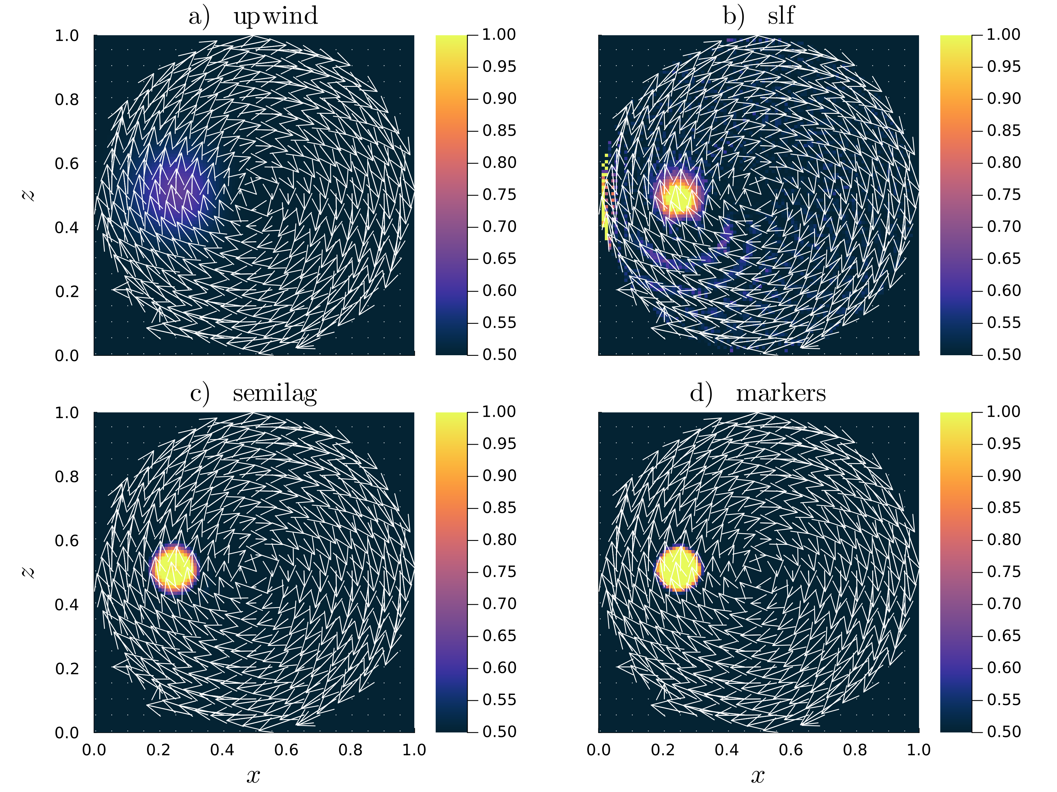
Figure 2. Summary. Final temperature distribution after one complete revolution for each advection scheme at a resolution of 100 × 100 cells.
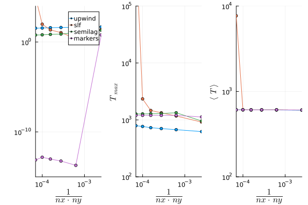
Figure 3. Advection Resolution Test. Relative deviation of the maximum temperature, final maximum temperature, and spatial mean temperature for the four advection schemes as functions of grid resolution.