Oceanic Geotherm
The 1-D temperature profile of an oceanic geotherm can be calculated by solving the conductive part of the 1-D temperature conservation equation using the conservative finite-difference solver for spatially variable thermal properties. Although constant thermal properties are assumed in this example, the variable-property solver is used to illustrate the more general formulation. For the sake of continuity, we use the 1-D solver for variable thermal properties, even though a constant thermal conductivity is assumed in this example.
In a conservative finite difference scheme for 1-D conduction, temperature is defined at the centroids, while vertical heat flux $q_y$ and thermal conductivity $k$ are defined at the vertices. This staggered arrangement ensures local conservation of heat by evaluating the divergence of the heat flux across the boundaries of each control volume.
The 1-D temperature equation is given by:
\[\begin{equation} \rho c_{p} \frac{\partial{T}}{\partial{t}} = \frac{\partial{q_y}}{\partial{y}} + \rho H, \end{equation}\]
where the heat flux is defined as:
\[\begin{equation} \left. q_{y,m} = -k_m \frac{\partial T}{\partial y}\right\vert_{m},\ \textrm{for}\ m = 1:nv, \end{equation}\]
where $\rho$, $c_{p}$, $T$, $t$, $k$, $H$, $y$, and $nv$ denote the density [kg/m³], the specific heat capacity [J/kg/K], the temperature [K], the time [s], the thermal conductivity [W/m/K], the heat generation rate per mass [W/kg], the depth [m], and the number of vertices, respectively.
For more details on how to discretize the equation using an explicit, forward Euler finite difference scheme, please see the documentation.
An additional script on how to solve the 1D heat diffusion equation using the combined, general solution (choosable discretization between explicit, implicit, and cna) for variable thermal properties can be found here.
First, one needs to load the required packages:
using Plots, SpecialFunctions
using GeoModBox.HeatEquation.OneD
Let's start with the definition of the geometrical, numerical, and physical constants:
# Constants --------------------------------------------------------- #
H           =   200e3               #   Height of the model [ m ]
nc          =   200                 #   Number of central grid points
Δy          =   H/nc                #   Grid resolution

# Depth ---
yc          =   LinRange(-H + Δy/2.0,0.0 - Δy/2.0,nc)
yv          =   LinRange(-H,0,nc+1)

Py  =   (
    ρm      =   3000,               #   Density [ kg/m^3 ]
    cpm     =   1000,               #   Heat capacity [ J/kg/K ]
    km      =   3.0,                #   Conductivity [ W/m/K ]
    HM      =   0,                  #   Heat generation rate [W/kg]; Q = ρ*H0
)
# ------------------------------------------------------------------- #
In the following, one needs to define the initial and boundary condition:
- Temperature at the surface and bottom.
- Linearly increasing temperature profile assuming a certain adiabatic gradient and potential mantle temperature.
# Initial Condition ------------------------------------------------- #
T   =   (
    Tpot    =   1315 + 273.15,      #   Potential temperature [ K ]
    ΔTadi   =   0.5,                #   Adiabatic temperature gradient [ K/km ]
    Ttop    =   273.15,             #   Surface temperature [ K ]
    T_ex    =   zeros(nc+2,1),
)
T1  =   (
    Tbot    =   T.Tpot + T.ΔTadi*abs(H/1e3),    # Bottom temperature [ K ]
    T       =   T.Tpot .+ abs.(yc./1e3).*T.ΔTadi,   # Initial T-profile [ K ]
)
T   =   merge(T,T1)

Tini                =   zeros(nc,1)
Tini                .=   T.T
T.T_ex[2:end-1]     .=   T.T
# ------------------------------------------------------------------- #
Either Dirichlet or Neumann thermal boundary conditions can be applied at the surface and bottom. Dirichlet boundary conditions are used throughout this example.
# Boundary conditions ----------------------------------------------- #
BC      =   (
    type    = (N=:Dirichlet, S=:Dirichlet),
    val     = (N=T.Ttop[1],S=T.Tbot[1])
)
# If Neumann boundary conditions are chosen, the following values result in the given heatflux for the given thermal conductivity k.
# S      =   -0.03;          # c     =   -k/q -> 90 mW/m^2
# N      =   -0.0033;        # c     =   -k/q -> 10 mW/m^2
# ------------------------------------------------------------------- #
Next, define the multiplicative factor fac for the diffusion stability criterion for the explicit thermal solver. This factor controls the stability criterion. If fac exceeds 1, the solver becomes unstable.
# Time stability criterion ------------------------------------------ #
fac     =   0.8
tmax    =   60                  #   Lithosphere age [ Ma ]
tsca    =   60*60*24*365.25     #   Seconds per year

age     =   tmax*1e6*tsca        #   Age in seconds
# ------------------------------------------------------------------- #
The initial temperature profile is plotted to verify that the initial and boundary conditions have been specified correctly.
# Plot Initial condition -------------------------------------------- #
plotparam   =   1
q = plot(Tini,yc./1e3,
    label="",
    xlabel="T [ K ]", ylabel="z [ km ]",
    title="Initial Temperature",
    xlim=(T.Ttop,T.Tbot),ylim=(-H/1e3,0))
display(q)
# ------------------------------------------------------------------- #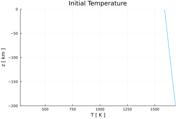
Figure 1. Initial temperature profile.
Although this example assumes constant material properties, the variable-property solver expects density, heat capacity, thermal conductivity, and radiogenic heat production to be defined as spatial fields. Therefore, the scalar material properties are expanded to vectors with the appropriate dimensions. The maximum thermal diffusivity is computed conservatively from the largest thermal conductivity and the smallest density and heat capacity. This value is used only for determining a stable explicit time step.
# Setup Fields ------------------------------------------------------ #
Py1     =   (
    ρ       =   Py.ρm.*ones(nc,1),
    cp      =   Py.cpm.*ones(nc,1),
    k       =   Py.km.*ones(nc+1,1),
    H       =   Py.HM.*ones(nc,1)
)
Py  =   merge(Py,Py1)
Py2     =   (
    # Thermal diffusivity [ m^2/s ]
    κ       =  maximum(Py.k)/minimum(Py.ρ)/minimum(Py.cp),
)
Py  =   merge(Py,Py2)
T2  =   (
    q   =   zeros(nc+1,1),
)
T   =   merge(T,T2)
# ------------------------------------------------------------------- #
Now, one can calculate the time stability criterion.
# Time stability criterion ------------------------------------------ #
Δtexp   =   Δy^2/2/Py.κ             #   Stability criterion for explicit
Δt      =   fac*Δtexp               #   total time step

nit     =   ceil(Int64,age/Δt)      #   Number of iterations

time    =   zeros(1,nit)            #   Time array
# ------------------------------------------------------------------- #
With all parameters and constants defined, the equation can now be solved the 1-D temperature equation for each time step in a for loop.
The temperature conservation equation is solved via the function ForwardEuler1D!(), which updates the temperature profile T.T for each time step using the extended temperature field T.T_ex, which include the ghost nodes. The temperature profile is plotted every 5 Myr to illustrate the thermal evolution of the oceanic lithosphere.
# Calculate 1-D temperature profile --------------------------------- #
count   =   1
for i = 1:nit
    if i > 1
        time[i]     =   time[i-1] + Δt
    elseif time[i] > age
        Δt          =   age - time[i-1]
        time[i]     =   time[i-1] + Δt
    end
    ForwardEuler1D!(T,Py,Δt,Δy,nc,BC)
    if i == nit || abs(time[i]/1e6/tsca - count*5.0) < Δt/1e6/tsca
        println(string("i = ",i,", time = ", time[i]/1e6/tsca))
        q = plot!(T.T,yc./1e3,
            label=string("t = ",ceil(time[i]/1e6/tsca),"[Ma]"),
            xlabel="T [ K ]", ylabel="z [ km ]",
            title="Oceanic Geotherm",
            xlim=(T.Ttop,T.Tbot),ylim=(-H/1e3,0))
        display(q)
        count = count + 1
    end
end
# ------------------------------------------------------------------- #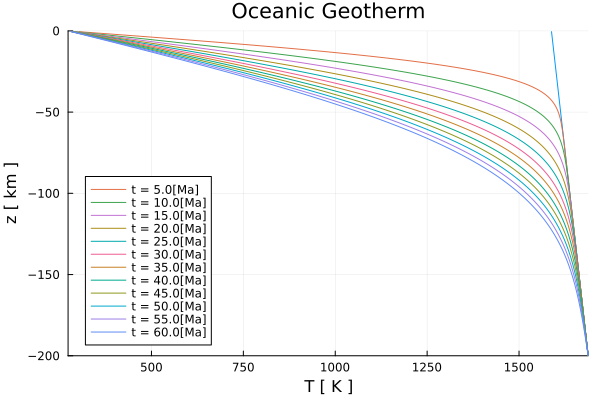
Figure 2. Evolution of the temperature profile with depth in 5 Ma steps.
Since the heat flux is defined at the grid vertices, the ghost-node temperatures are first updated according to the prescribed boundary conditions before Fourier's law is evaluated.
# Calculate heat flow ----------------------------------------------- #
# South ---
T.T_ex[1]   =   (BC.type.S==:Dirichlet) * (2 * BC.val.S - T.T_ex[2]) +
                (BC.type.S==:Neumann) * (T.T_ex[2] - BC.val.S*Δy)
# North ---
T.T_ex[end] =   (BC.type.N==:Dirichlet) * (2 * BC.val.N - T.T_ex[nc+1]) +
                (BC.type.N==:Neumann) * (T.T_ex[nc+1] + BC.val.N*Δy)
for j=1:nc+1
    T.q[j]  =   -Py.k[j] *
        (T.T_ex[j+1] - T.T_ex[j])/Δy
end
# ------------------------------------------------------------------- #
Finally, compute the temperature profile for an oceanic geotherm using the analytical solution of the infinite half-space cooling model (HSCM) for a certain age. The numerical solution is compared with the analytical HSCM solution, providing a useful verification of the numerical implementation. The initial condition is a linear adiabatic profile and the HSCM solution is superimposed onto this reference profile.
# Plot -------------------------------------------------------------- #
if BC.type.N==:Dirichlet && BC.type.S==:Dirichlet
    Tana    =   zeros(nc,1)
    Tana    .=   Tini .+ (T.Ttop - T.Tpot).*erfc.(-yc./(2*sqrt(age*Py.κ)))
    Tana[end] =   T.Ttop
end
p = plot(T.T,yc./1e3,
        label=string("t = ",ceil(maximum(time)/1e6/tsca),"[Ma]"),
        xlabel="T [ K ]", ylabel="z [ km ]",
        title="Oceanic Geotherm",
        xlim=(T.Ttop,T.Tbot),ylim=(-H/1e3,0),
        layout=(1,2),subplot=1)
if BC.type.N==:Dirichlet && BC.type.S==:Dirichlet
    plot!(p,Tana,yc./1e3,
            label="T_HSCM",linestyle=:dash,
            layout=(1,2),subplot=1)
end
p = plot!(T.q.*1e3,yv./1e3,
        label="",
        xlabel="q [ mW ]", ylabel="z [m]",
        title="Heat Flux",
        ylim=(-H/1e3,0),
        subplot=2)
display(p)
savefig(p,"./examples/DiffusionEquation/1D/Results/OceanicGeotherm_1D.png")
savefig(q,"./examples/DiffusionEquation/1D/Results/OceanicGeotherm_1D_evolve.png")
# ======================================================================= #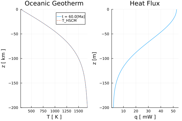
Figure 3. Comparison between the numerical and analytical half-space cooling solutions together with the corresponding vertical heat-flux profile.