Falling Block Benchmark
The falling block benchmark is a well-established test for assessing the accuracy of the momentum solver and the efficiency of the advection scheme, particularly under strong viscosity and density contrasts (Gerya, 2019). The model setup (Figure 1) is defined by a rectangular block with a certain viscosity and density within a matrix of a different viscosity and density. Due to the density contrast, the block sinks. Depending on the viscosity contrast, the block either deforms strongly during its descent or behaves nearly as a rigid body. Consequently, the benchmark simultaneously tests the treatment of large viscosity contrasts and the accuracy of material advection.
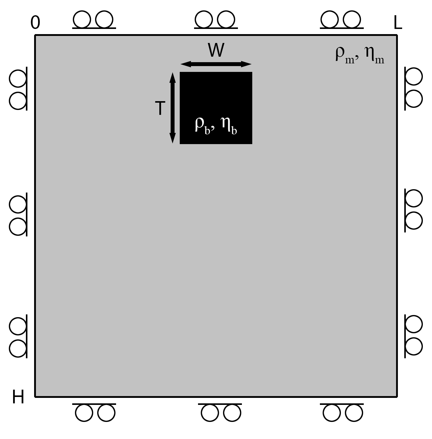
Figure 1. Falling Block Setup.
The purpose of this benchmark is twofold:
Accuracy of the variable viscosity momentum solver. Solving the momentum equation for the initial state, one can calculate the sinking velocity of the block, which follows a characteristic trend as a function of the viscosity contrast between the block and the matrix.
Accuracy of the advection scheme. Assuming a time-dependent problem, one can test the efficiency of the advection scheme. Here, all four different advection schemes can be chosen:
- Upwind
- Staggered leapfrog
- Semi-Lagrangian
- Tracers
In the tracer method, each marker carries the complete set of material properties (phase, density, viscosity, etc.), which are interpolated back to the numerical grid after advection. For the Eulerian advection scheme, only the phase is advected along the centroids. The material parameters on the centroids are updated using the phase ratio at each centroids.Density is reconstructed by linear interpolation between the material densities, whereas viscosity is reconstructed using the selected viscosity averaging scheme. Tests with harmonic and geometric viscosity averaging produced substantially smaller stable timesteps, particularly for weak inclusions. This results from the strong influence of intermediate phase fractions on the effective viscosity and substantially increases the required number of Stokes solves. Arithmetic averaging is therefore used as the default for this example because it provides the most robust and computationally practical behavior over the investigated viscosity contrasts. This choice is specific to the present discretization, phase-field reconstruction, and benchmark configuration; it should not be interpreted as a general preference for arithmetic viscosity averaging in all multiphase Stokes-flow problems.
Note: In its current implementation, the staggered leapfrog scheme is not well suited for advecting discontinuous phase fields. Although clamping prevents unphysical phase values, the dispersive nature of the leapfrog scheme produces oscillatory interfaces that significantly degrade the solution quality. The semi-Lagrangian method performs considerably better but becomes computationally expensive for large viscosity contrasts because it requires substantially smaller timesteps than the other advection methods.
This example solves the falling block benchmark across a viscosity contrast range spanning six orders of magnitude (from $10^{-6}$ to $10^6$). The simulation yields either the block’s initial sinking velocity (for steady-state problems; td = 0), or its final position (for time-dependent problems with a viscosity ratio $\eta_r \geq 0$, td = 1). For additional information on the benchmark, please refer to the exercise. This example uses the specialized direct Stokes solver provided by GeoModBox.jl. An equivalent implementation based on the general defect correction solver is available separately. Both implementations solve the same benchmark problem and produce equivalent solutions for the prescribed linear viscosity field, while illustrating two different solver interfaces.
Again, the output of the script depends on the definition of the parameter save_fig.
save_fig = 0- Output every plot for each time step and model (not recommended!)save_fig = 1- Save the animations for each model and store the final position (if the issue is steady state, this stores the sinking velocity plot)save_fig = -1- Only store the final position for a time-dependent problem
Let's first load the required modules.
using Plots
using ExtendableSparse
using GeoModBox.InitialCondition, GeoModBox.MomentumEquation.TwoD
using GeoModBox.AdvectionEquation.TwoD
using GeoModBox.Tracers.TwoD
using Base.Threads
using Printf
For the Eulerian advection schemes, only the phase ratio is transported. The density and viscosity fields are reconstructed after each advection step using the transported phase ratio. The helper function below performs this reconstruction.
function UpdateRheology!(D,ρ,η,avg)
    # Density --- artihmetic averaging ---
    @. D.ρ     =   ρ[1]*(1.0 - D.p) + ρ[2]*D.p
    D.ρ_ex[2:end-1,2:end-1]     .=  D.ρ
    D.ρ_ex[1,:]     .=  D.ρ_ex[2,:]
    D.ρ_ex[end,:]   .=  D.ρ_ex[end-1,:]
    D.ρ_ex[:,1]     .=  D.ρ_ex[:,2]
    D.ρ_ex[:,end]   .=  D.ρ_ex[:,end-1]
    # Viscosity - Centroids and vertices ---
    if avg ==     :arithmetic
        @. D.ηc =   (1.0 - D.p) * η[1] + D.p * η[2]
    elseif avg == :harmonic
        @. D.ηc =   1.0 / ( (1.0 - D.p) / η[1] + D.p / η[2] )
    elseif avg == :geometric
        @. D.ηc =   η[1]^(1.0 - D.p) * η[2]^D.p
    else
        error("Unknown viscosity averaging: $(avg)")
    end
    # --- Extended Centroids-
    D.η_ex[2:end-1,2:end-1]     .=  D.ηc
    D.η_ex[1,:]     .=  D.η_ex[2,:]
    D.η_ex[end,:]   .=  D.η_ex[end-1,:]
    D.η_ex[:,1]     .=  D.η_ex[:,2]
    D.η_ex[:,end]   .=  D.η_ex[:,end-1]
    # --- Vertices -
    if avg == :arithmetic
        @. D.ηv =
            0.25*(
                D.η_ex[1:end-1,1:end-1] +
                D.η_ex[2:end  ,1:end-1] +
                D.η_ex[1:end-1,2:end  ] +
                D.η_ex[2:end  ,2:end  ]
            )
    elseif avg == :harmonic
        @. D.ηv =
            4.0/(
                1/D.η_ex[1:end-1,1:end-1] +
                1/D.η_ex[2:end  ,1:end-1] +
                1/D.η_ex[1:end-1,2:end  ] +
                1/D.η_ex[2:end  ,2:end  ]
            )
    elseif avg == :geometric
        @. D.ηv =
            exp(0.25*(
                log(D.η_ex[1:end-1,1:end-1]) +
                log(D.η_ex[2:end  ,1:end-1]) +
                log(D.η_ex[1:end-1,2:end  ]) +
                log(D.η_ex[2:end  ,2:end  ])
            ))
    else
        error("Unknown viscosity averaging: $(avg)")
    end

    return D

end
# ======================================================================= #
In the following, one can define the range of the viscosity ratios to be calculated and the maximum time is set for each model assuming a viscosity ratio from -6 to 6 orders of magnitude. Additionally, one can define it the problem should be steady-state or time-dependent.
# Make it time-dependent (1) or steady-state (0)
td      =   0
to      =   TimerOutput()
@timeit to "Ini" begin
# Benchmark parameter =============================================== #
ηᵣ      =   LinRange(-6.0,6.0,13)       #   Viscosity ratio
sv      =   zeros(length(ηᵣ))           #   Sinking Velocity
tmax    =   [7.115094, 7.114844, 7.256534, 7.377311, 7.738412,
                7.673613, 9.886, 15.446, 19.623, 20.569, 20.569,
                20.569, 20.589]
# ------------------------------------------------------------------- #
In the following, one can define the advection scheme and the initial configuration. For more details on how the initial condition is implemented in GeoModBox.jl, please refer to the documentation.
# Define Numerical Scheme =========================================== #
# Advection ---
#   1) upwind, 2) slf, 3) semilag, 4) tracers
# Advection methods:
#
# :tracers
#     Recommended for this benchmark. Preserves the sharp material
#     interface and remains robust for large viscosity contrasts.
#
# :semilag
#     Produces a comparatively coherent interface but requires bounded
#     phase values and careful departure-point boundary treatment.
#
# :upwind
#     Robust and bounded, but strongly diffuses the material interface.
#
# :slf
#     Not recommended for discontinuous phase fields because dispersive
#     oscillations and the leapfrog computational mode destabilize the
#     interface.
FD          =   (Method     = (Adv=:tracers,),)
# Arithmetic averaging is used for this benchmark because harmonic and
# geometric mixing produce strongly reduced mixed-cell viscosities for
# weak inclusions. In combination with semi-Lagrangian phase transport,
# this leads to large local velocities, very small CFL timesteps, and a
# substantial increase in the required number of Stokes solves.
#
# This is an implementation-specific choice and not a general statement
# that arithmetic viscosity averaging is optimal for all multiphase
# Stokes problems.
avg         =   :arithmetic
avgm        =   :arith
# ------------------------------------------------------------------- #
# Define Initial Condition ========================================== #
# Density ---
#   1) block
Ini         =   (p=:block,)
# ------------------------------------------------------------------- #
Now, one can set the directory to save the animaion to and some plotting parameters.
# Animation and Plot Settings ======================================= #
path        =   string("./examples/StokesEquation/2D/Results/")
save_fig    =   1
p2          =   plot(0,0,layout=(2,3))
count       =   Int64(0)
panel       =   ["(a)","(b)","(c)","(d)","(e)","(f)",]
# ------------------------------------------------------------------- #
# Plot Settings ===================================================== #
Pl  =   (
    qinc    =   1,
    qsc     =   100*(60*60*24*365.25)*5e1
)
# ------------------------------------------------------------------- #
In the following, one defines the model geometry and the numerical grid parameters.
# Geometry ========================================================== #
M       =   (
    xmin    =   0.0,
    xmax    =   500.0e3,    # [ m ]
    ymin    =   -500.0e3,   # [ m ]
    ymax    =   0.0,
)
# ------------------------------------------------------------------- #
# Grid ============================================================== #
NC      =   (
    x   =   50,
    y   =   50,
)
NV      =   (
    x   =   NC.x + 1,
    y   =   NC.y + 1,
)
Δ       =   (
    x   =   (M.xmax - M.xmin)/NC.x,
    y   =   (M.ymax - M.ymin)/NC.y,
)
x       =   (
    c   =   LinRange(M.xmin+Δ.x/2,M.xmax-Δ.x/2,NC.x),
    ce  =   LinRange(M.xmin - Δ.x/2.0, M.xmax + Δ.x/2.0, NC.x+2),
    v   =   LinRange(M.xmin,M.xmax,NV.x),
)
y       =   (
    c   =   LinRange(M.ymin+Δ.y/2,M.ymax-Δ.y/2,NC.y),
    ce  =   LinRange(M.ymin - Δ.y/2.0, M.ymax + Δ.y/2.0, NC.y+2),
    v   =   LinRange(M.ymin,M.ymax,NV.y),
)
x1      =   (
    c2d     =   x.c .+ 0*y.c',
    v2d     =   x.v .+ 0*y.v',
    vx2d    =   x.v .+ 0*y.ce',
    vy2d    =   x.ce .+ 0*y.v',
)
x   =   merge(x,x1)
y1      =   (
    c2d     =   0*x.c .+ y.c',
    v2d     =   0*x.v .+ y.v',
    vx2d    =   0*x.v .+ y.ce',
    vy2d    =   0*x.ce .+ y.v',
)
y   =   merge(y,y1)
# ------------------------------------------------------------------- #
Now, one can set the physical constants of the problem. The arrays ρ and phase are used to advect the material. For more information on how this is implemented, please refer to the documentation. Additionally, the velocity boundary conditions are set.
# Physics =========================================================== #
g       =   9.81                #   Gravitational Acceleration

η₀      =   1.0e21              #   Background Viscosity

ρ₀      =   3200.0              #   Background density
ρ₁      =   3300.0              #   Block density
ρ       =   [ρ₀,ρ₁]             #   Density for phases

phase   =   [0,1]               #   Phase ID
# ------------------------------------------------------------------- #
# Boundary Conditions =============================================== #
VBC     =   (
    type    =   (E=:freeslip,W=:freeslip,S=:freeslip,N=:freeslip),
    val     =   (E=zeros(NV.y),W=zeros(NV.y),S=zeros(NV.x),N=zeros(NV.x),
                vxE=zeros(NC.y),vxW=zeros(NC.y),vyS=zeros(NC.x),vyN=zeros(NC.x)),
)
# ------------------------------------------------------------------- #
Now, one can start the loop of the different viscosity ratio.
@timeit to "η loop" begin
    for mn in eachindex(ηᵣ)     #   Loop over ηᵣ
To store the animation of each model, the name of the gif file is defined in the following.
    anim        =   Plots.Animation(path, String[] )
    filename    =   string("Falling_",Ini.p,"_ηr_",round(ηᵣ[mn]),
                        "_",FD.Method.Adv,"_direct_",avg)
    # --------------------------------------------------------------- #
Now, one can set the viscosity for the block and the viscosity array η for the advection scheme.
    # Physics ======================================================= #
    η₁      =   η₀ * 10^(ηᵣ[mn])    #   Block Viscosity
    η       =   [η₀,η₁]             #   Viscosity for phases
    @show η
    # --------------------------------------------------------------- #
In the following, the data arrays are initialized.
    # Allocation ==================================================== #
    D   =   (
        vx      =   zeros(Float64,NV.x,NC.y+2),
        vy      =   zeros(Float64,NC.x+2,NV.y),
        Pt      =   zeros(Float64,NC...),
        p       =   zeros(Float64,NC...),
        p_ex    =   zeros(Float64,NC.x+2,NC.y+2),
        p_exo   =   zeros(Float64,NC.x+2,NC.y+2),
        ρ       =   zeros(Float64,NC...),
        ρ_ex    =   zeros(Float64,NC.x+2,NC.y+2),
        ρ_exo   =   zeros(Float64,NC.x+2,NC.y+2),
        vxc     =   zeros(Float64,NC...),
        vyc     =   zeros(Float64,NC...),
        vxco    =   zeros(Float64,NC...),
        vyco    =   zeros(Float64,NC...),
        vc      =   zeros(Float64,NC...),
        wt      =   zeros(Float64,(NC.x,NC.y)),
        wte     =   zeros(Float64,(NC.x+2,NC.y+2)),
        wtv     =   zeros(Float64,(NV.x,NV.y)),
        ηc      =   zeros(Float64,NC...),
        ηv      =   zeros(Float64,NV...),
        η_ex    =   zeros(Float64,NC.x+2,NC.y+2),
        η_exo   =   zeros(Float64,NC.x+2,NC.y+2),
    )
    # --------------------------------------------------------------- #
Now, one needs to initialize the time parameters.
if FD.Method.Adv==:semilag
        Δfac    =   0.25
    else
        Δfac    =   0.9
    end
    T   =   (
        tmax    =   [0.0],
        Δfac    =   Δfac,    # Courant time factor, i.e. dtfac*dt_courant
        Δ       =   [0.0],
        time    =   [0.0,0.0],
    )
    T.tmax[1]   =   tmax[mn] * 1e6 * (60*60*24*365.25)   # [ s ]
    if td == 0
        nt  =   1
    else
        nt  =   9999
    end
    # --------------------------------------------------------------- #
In case tracers are used, the tracers are initialized in the following. Alternatively, the initial density and viscosity are defined on the extended grid using the phase distribution. For more details on the initial conditions, please refer to the documentation.
    # Tracer Advection ============================================== #
    if FD.Method.Adv==:tracers
        @timeit to "Tracer Ini" begin
        # Tracer Initialization ---
        nmx,nmy     =   3,3
        noise       =   0
        nmark       =   nmx*nmy*NC.x*NC.y
        Aparam      =   :phase
        MPC         =   (
                c       =   zeros(Float64,(NC.x,NC.y)),
                v       =   zeros(Float64,(NV.x,NV.y)),
                th      =   zeros(Float64,(nthreads(),NC.x,NC.y)),
                thv     =   zeros(Float64,(nthreads(),NV.x,NV.y)),
        )
        MAVG        = (
                PC_th   =   [similar(D.wte) for _ = 1:nthreads()],  # per thread
                PV_th   =   [similar(D.ηv) for _ = 1:nthreads()],   # per thread
                wte_th  =   [similar(D.wte) for _ = 1:nthreads()],  # per thread
                wtv_th  =   [similar(D.wtv) for _ = 1:nthreads()],  # per thread
        )
        Ma      =   IniTracer2D(Aparam,nmx,nmy,Δ,M,NC,noise,Ini.p,phase)
        # RK4 weights ---
        rkw     =   1.0/6.0*[1.0 2.0 2.0 1.0]   # for averaging
        rkv     =   1.0/2.0*[1.0 1.0 2.0 2.0]   # for time stepping
        # Count marker per cell ---
        CountMPC(Ma,nmark,MPC,M,x,y,Δ,NC,NV)
        # Interpolate from markers to cell ---
        Markers2Cells(Ma,nmark,MAVG.PC_th,D.ρ_ex,MAVG.wte_th,D.wte,x,y,Δ,Aparam,ρ)
        D.ρ     .=  D.ρ_ex[2:end-1,2:end-1]
        Markers2Cells(Ma,nmark,MAVG.PC_th,D.p_ex,MAVG.wte_th,D.wte,x,y,Δ,Aparam,phase)
        D.p     .=  D.p_ex[2:end-1,2:end-1]
        Markers2Cells(Ma,nmark,MAVG.PC_th,D.η_ex,MAVG.wte_th,D.wte,x,y,Δ,Aparam,η;avgm=avgm)
        D.ηc    .=  D.η_ex[2:end-1,2:end-1]
        Markers2Vertices(Ma,nmark,MAVG.PV_th,D.ηv,MAVG.wtv_th,D.wtv,x,y,Δ,Aparam,η;avgm=avgm)
        end
    else
        @timeit to "Phase Ini" begin
        # ----------------------------------------------------------- #
        # Initial Condition ========================================= #
        IniPhase!(Ini.p,D,M,x,y,NC;phase)
        UpdateRheology!(D,ρ,η,avg)
        end
    end
    # --------------------------------------------------------------- #
Now, one needs to define the parameters for the linear system of equations of the momentum equation.
    # System of Equations =========================================== #
    # Numbering, without ghost nodes! ---
    off    = [  NV.x*NC.y,                          # vx
                NV.x*NC.y + NC.x*NV.y,              # vy
                NV.x*NC.y + NC.x*NV.y + NC.x*NC.y]  # Pt

    Num    =    (
        Vx  =   reshape(1:NV.x*NC.y, NV.x, NC.y),
        Vy  =   reshape(off[1]+1:off[1]+NC.x*NV.y, NC.x, NV.y),
        Pt  =   reshape(off[2]+1:off[2]+NC.x*NC.y,NC...),
    )
    # --------------------------------------------------------------- #
Let's start the time loop!
    @timeit to "Time Loop" begin
    # Time Loop ===================================================== #
    for it = 1:nt
First, the unknown and right-hand vector for the system of equations are defined.
        χ       =   zeros(maximum(Num.Pt))      #   Unknown Vector
        rhs     =   zeros(maximum(Num.Pt))      #   Right-hand Side
        # Update Time ---
        T.time[1]   =   T.time[2]
        @printf("Time step: #%04d, Time [Myr]: %04e\n ",it,
                    T.time[1]/(60*60*24*365.25)/1.0e6)
Now, one can solve the system of equations, for example, using the direct method. For more information on how this is solved, please refer to the documentation. To advect the material using the first three advection scheme, the centroid velocity is calculated.
        # Momentum Equation =======
        # Update K ---
        @timeit to "Assembly" begin
        K       =   Assembly( NC, NV, Δ, D.ηc, D.ηv, VBC, Num )
        end
        # Update RHS ---
        @timeit to "Update RHS" begin
        rhs     =   updaterhs( NC, NV, Δ, D.ηc, D.ηv, D.ρ, g, VBC, Num )
        end
        # Solve System of Equations ---
        @timeit to "Solution" begin
        χ       =   K \ rhs
        end
        # Update Unknown Variables ---
        D.vx[:,2:end-1]     .=  χ[Num.Vx]
        D.vy[2:end-1,:]     .=  χ[Num.Vy]
        D.Pt                .=  χ[Num.Pt]
        # ======
        # Get the velocity on the centroids ---
        for i = 1:NC.x
            for j = 1:NC.y
                D.vxc[i,j]  = (D.vx[i,j+1] + D.vx[i+1,j+1])/2
                D.vyc[i,j]  = (D.vy[i+1,j] + D.vy[i+1,j+1])/2
            end
        end
        if FD.Method.Adv==:semilag
            if it == 1
                @. D.vxco   =   D.vxc
                @. D.vyco   =   D.vyc
            end
        end
        @. D.vc        = sqrt(D.vxc^2 + D.vyc^2)
        # ---
        if it == 1
            sv[mn]  =   maximum(D.vc)
        end
        # ---
        if T.time[2] >= T.tmax[1]
            it = nt
        end
        # ---
In the following, the figures for each time step are plotted. The style of the plot varies depending on the advection scheme.
        if mod(it,2) == 0 || it == nt || it == 1
            if FD.Method.Adv==:tracers
                p = heatmap(x.c./1e3,y.c./1e3,D.p',color=:inferno,
                            xlabel="x[km]",ylabel="y[km]",colorbar=false,
                            title="Phase_c",
                            aspect_ratio=:equal,xlims=(M.xmin/1e3, M.xmax/1e3),
                            ylims=(M.ymin/1e3, M.ymax/1e3),
                            layout=(2,2),subplot=1)
            else
                p = heatmap(x.v./1e3,y.v./1e3,log10.(abs.(D.ηv')),color=reverse(cgrad(:roma)),
                            xlabel="x[km]",ylabel="y[km]",title="η_v",
                            clims=(15,27),
                            aspect_ratio=:equal,xlims=(M.xmin/1e3, M.xmax/1e3),
                            ylims=(M.ymin/1e3, M.ymax/1e3),colorbar=true,
                            layout=(2,2),subplot=1)
            end
            if FD.Method.Adv==:tracers
                scatter!(p,Ma.x[1:Pl.qinc:end]./1e3,Ma.y[1:Pl.qinc:end]./1e3,
                            ms=1,ma=0.5,mc=Ma.phase[1:Pl.qinc:end],markerstrokewidth=0.0,
                            xlabel="x[km]",ylabel="y[km]",colorbar=false,
                            title="tracers",label="",
                            aspect_ratio=:equal,xlims=(M.xmin/1e3, M.xmax/1e3),
                            ylims=(M.ymin/1e3, M.ymax/1e3),
                            layout=(2,2),subplot=2)
            else
                heatmap!(p,x.c./1e3,y.c./1e3,D.ρ',color=:inferno,
                            xlabel="x[km]",ylabel="y[km]",colorbar=false,
                            title="Density",
                            aspect_ratio=:equal,xlims=(M.xmin/1e3, M.xmax/1e3),
                            ylims=(M.ymin/1e3, M.ymax/1e3),
                            layout=(2,2),subplot=2)
            end
            heatmap!(p,x.c./1e3,y.c./1e3,D.vc',
                        xlabel="x[km]",ylabel="y[km]",colorbar=false,
                        title="V_c",color=cgrad(:batlow),
                        aspect_ratio=:equal,xlims=(M.xmin/1e3, M.xmax/1e3),
                        ylims=(M.ymin/1e3, M.ymax/1e3),
                        layout=(2,2),subplot=4)
            quiver!(p,x.c2d[1:Pl.qinc:end,1:Pl.qinc:end]./1e3,
                        y.c2d[1:Pl.qinc:end,1:Pl.qinc:end]./1e3,
                        quiver=(D.vxc[1:Pl.qinc:end,1:Pl.qinc:end].*Pl.qsc,
                                D.vyc[1:Pl.qinc:end,1:Pl.qinc:end].*Pl.qsc),
                        la=0.5,color="white",layout=(1,3),subplot=3)
            heatmap!(p,x.c./1e3,y.c./1e3,log10.(abs.(D.ηc)'),color=reverse(cgrad(:roma)),
                        xlabel="x[km]",ylabel="y[km]",title="η_c",
                        clims=(15,27),
                        aspect_ratio=:equal,xlims=(M.xmin/1e3, M.xmax/1e3),
                        ylims=(M.ymin/1e3, M.ymax/1e3),colorbar=true,
                        layout=(2,2),subplot=3)
            if save_fig == 1
                Plots.frame(anim)
            elseif save_fig == 0
                display(p)
            end
        end
        if T.time[2] >= T.tmax[1]
            break
        end
Now, one needs to calculate the time step to advect the material.
        # Calculate Time Stepping ---
        T.Δ[1]      =   T.Δfac * minimum((Δ.x,Δ.y)) /
                            (sqrt(maximum(abs.(D.vx))^2 + maximum(abs.(D.vy))^2))
        # ---
        @printf("\n")
        # Calculate Time ---
        T.time[2]   =   T.time[1] + T.Δ[1]
        if T.time[2] > T.tmax[1]
            T.Δ[1]      =   T.tmax[1] - T.time[1]
            T.time[2]   =   T.time[1] + T.Δ[1]
        end
In the following the advection is conducted. For more details on this, please refer to the documentation.
    # Advection ======
        if FD.Method.Adv==:upwind
            upwindc2D!(D.p,D.p_ex,D.vxc,D.vyc,NC,T.Δ[1],Δ.x,Δ.y)
        elseif FD.Method.Adv==:slf
            slfc2D!(D.p,D.p_ex,D.p_exo,D.vxc,D.vyc,NC,T.Δ[1],Δ.x,Δ.y)
        elseif FD.Method.Adv==:semilag
            semilagc2D!(D.p,D.p_ex,D.vxc,D.vyc,D.vxco,D.vyco,x,y,T.Δ[1])
        elseif FD.Method.Adv==:tracers
            # Advect tracers ---
            @printf("Running on %d thread(s)\n", nthreads())
            AdvectTracer2D(Ma,nmark,D,x,y,T.Δ[1],Δ,NC,rkw,rkv)
            CountMPC(Ma,nmark,MPC,M,x,y,Δ,NC,NV)
            # Interpolate phase from tracers to grid ---
            Markers2Cells(Ma,nmark,MAVG.PC_th,D.ρ_ex,MAVG.wte_th,D.wte,x,y,Δ,Aparam,ρ)
            D.ρ     .=   D.ρ_ex[2:end-1,2:end-1]
            Markers2Cells(Ma,nmark,MAVG.PC_th,D.p_ex,MAVG.wte_th,D.wte,x,y,Δ,Aparam,phase)
            D.p     .=  D.p_ex[2:end-1,2:end-1]
            Markers2Cells(Ma,nmark,MAVG.PC_th,D.η_ex,MAVG.wte_th,D.wte,x,y,Δ,Aparam,η;avgm=avgm)
            D.ηc    .=   D.η_ex[2:end-1,2:end-1]
            Markers2Vertices(Ma,nmark,MAVG.PV_th,D.ηv,MAVG.wtv_th,D.wtv,x,y,Δ,Aparam,η;avgm=avgm)
        end
        if FD.Method.Adv!=:tracers
            @. D.p      = clamp(D.p, 0.0, 1.0)
            @. D.p_ex   = clamp(D.p_ex, 0.0, 1.0)
            @. D.p_exo  = clamp(D.p_exo, 0.0, 1.0)
            UpdateRheology!(D,ρ,η,avg)
        end
        @printf("\n")
        if FD.Method.Adv==:semilag
            @. D.vxco   =   D.vxc
            @. D.vyco   =   D.vyc
        end
        # D.p_exo     .=  D.p_ex
    end     # End Time Loop
    end
If requested, the final position of the blocks are plotted and stored in the following.
    if ηᵣ[mn] == 0.0 || ηᵣ[mn] == 1.0 || ηᵣ[mn] == 2.0 ||
                        ηᵣ[mn] == 3.0 || ηᵣ[mn] == 4.0 || ηᵣ[mn] == 6.0
        count = count + 1
        if FD.Method.Adv==:tracers
            if ηᵣ[mn] == 3.0 || ηᵣ[mn] ==  4.0 || ηᵣ[mn] == 6.0
                xlab    =   L"x[km]"
                xf      =   :auto
            else
                xlab    =   ""
                xf      =   _ -> ""
            end
            if ηᵣ[mn] == 0.0 || ηᵣ[mn] == 3.0
                ylab    =   L"y[km]"
                yf      =   :auto
            else
                ylab    =   ""
                yf      =   _ -> ""
            end
            p2  =   scatter!(p2,Ma.x[1:Pl.qinc:end]./1e3,Ma.y[1:Pl.qinc:end]./1e3,
                ms=2,ma=0.5,mc=Ma.phase[1:Pl.qinc:end],markerstrokewidth=0.0,
                xlabel=xlab,ylabel= ylab,colorbar=false,
                title           = latexstring(panel[count],"\\quad\\log_{10}(\\eta_r)=",string(ηᵣ[mn])),
                titlefontsize   = 20,
                label="", xformatter = xf,yformatter = yf,
                aspect_ratio=:equal,xlims=(M.xmin/1e3, M.xmax/1e3),
                ylims=(M.ymin/1e3, M.ymax/1e3),
                layout=(2,3),subplot=count,
                framestyle      = :box,
                guidefontsize   = 20,
                tickfontsize    = 16,
                size            = (1200, 800),
                right_margin    = 8mm,
                left_margin     = 8mm,
                dpi             = 300)
        else
            p2 = heatmap!(p2,x.c./1e3,y.c./1e3,D.p',color=:inferno,
                xlabel="x[km]",ylabel="y[km]",colorbar=false,
                title="Phase_c",
                aspect_ratio=:equal,xlims=(M.xmin/1e3, M.xmax/1e3),
                ylims=(M.ymin/1e3, M.ymax/1e3),
                layout=(2,3),subplot=count)
        end
    end
    # Save Animation ---
    if save_fig == 1
        if td == 1
            # Write the frames to a GIF file
            Plots.gif(anim, string( path, filename, ".gif" ), fps = 15)
            foreach(rm, filter(startswith(string(path,"00")), readdir(path,join=true)))
        end
    end
end # End ηᵣ Loop
end
In case the problem is set to be steady-state, the sinking velocity is plotted. If the problem is time-dependent the final position is stored.
if td == 0
        q = scatter(ηᵣ,sv.*(100.0*365.25*24*60*60),
                        ylabel          = L"v_\mathrm{block} [cm/a]",
                        xlabel          = L"log_{10}\left(\eta_\mathrm{b}/\eta_\mathrm{m}\right)",
                        title           = "Sinking Velocity",
                        label           = false,
                        marker          = :circle,
                        markersize      = 7,
                        markercolor     = :black,
                        markerstrokecolor = :black,
                        markerstrokewidth = 0.8,
                        framestyle      = :box,
                        grid            = false,
                        guidefontsize   = 20,
                        tickfontsize    = 16,
                        legendfontsize  = 14,
                        xlims           = (-6, 6),
                        ylims           = (1.0, 5.0),
                        xticks          = -6:2:6,
                        size            = (900, 650),
                        left_margin     = 5mm,
                        right_margin    = 5mm,
                        bottom_margin   = 5mm,
                        top_margin      = 5mm,
                        dpi             = 300,)
        plot!(
            q,
            ηᵣ,
            sv .*(100.0*365.25*24*60*60),
            color      = :black,
            linewidth  = 2.0,
            linestyle  = :solid,
            label      = false,
        )
        if save_fig == 1
            savefig(q,string("./examples/StokesEquation/2D/Results/FallingBlock_SinkingVeloc",
                                "_",FD.Method.Adv,"_direct_",avg,".png"))
            foreach(rm, filter(startswith(string(path,"00")), readdir(path,join=true)))
        else
            display(q)
        end
    else
        if save_fig == -1 ||save_fig == 1
            savefig(p2,string("./examples/StokesEquation/2D/Results/FallingBlock_FinalStage",
                                "_",FD.Method.Adv,"_direct_",avg,".png"))
        else
            display(p2)
        end
    end
    display(to)
end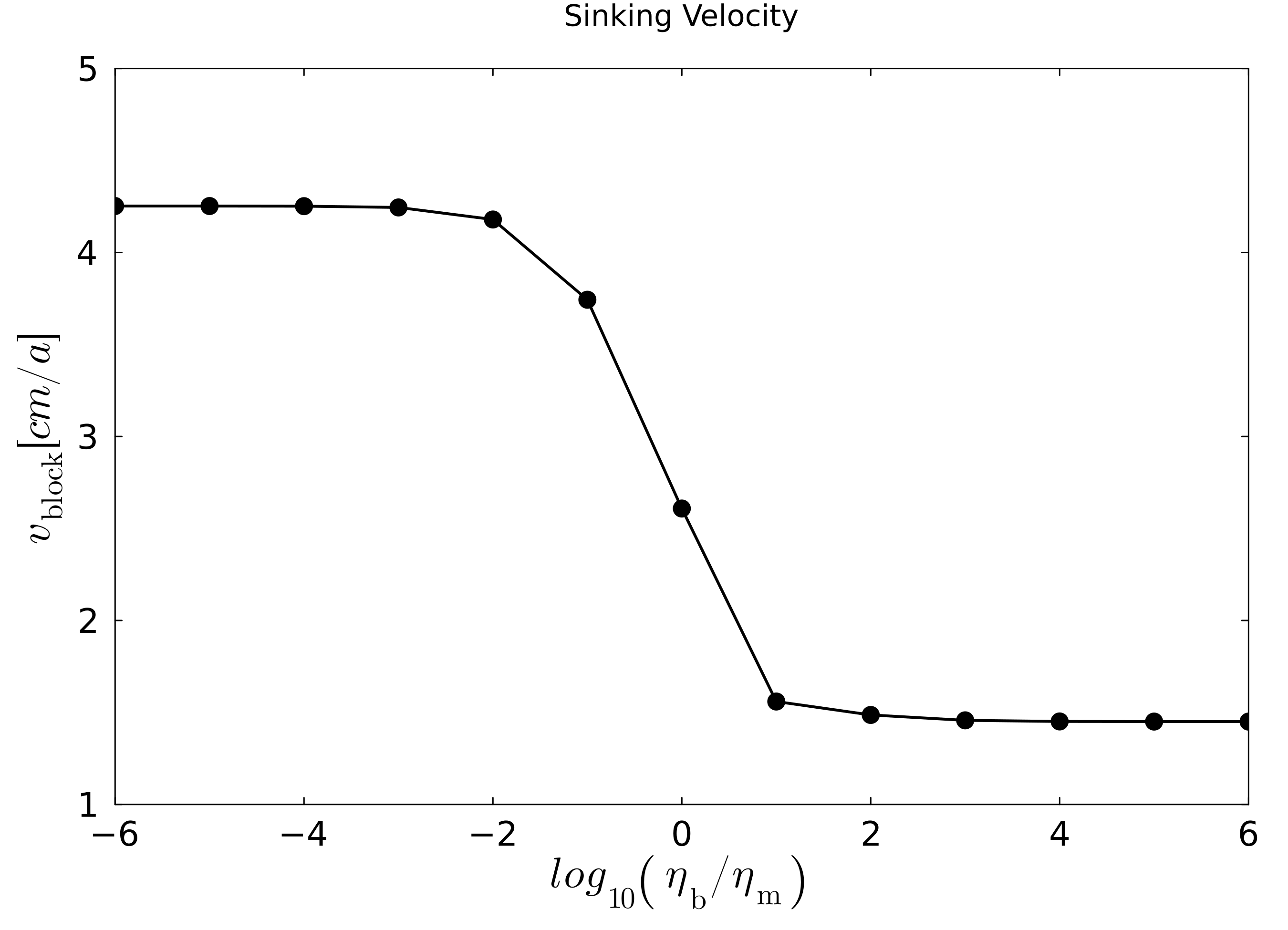
Figure 2. Sinking Velocity. Instantaneous, sinking velocity of the rectangular block for different viscosity ratios.
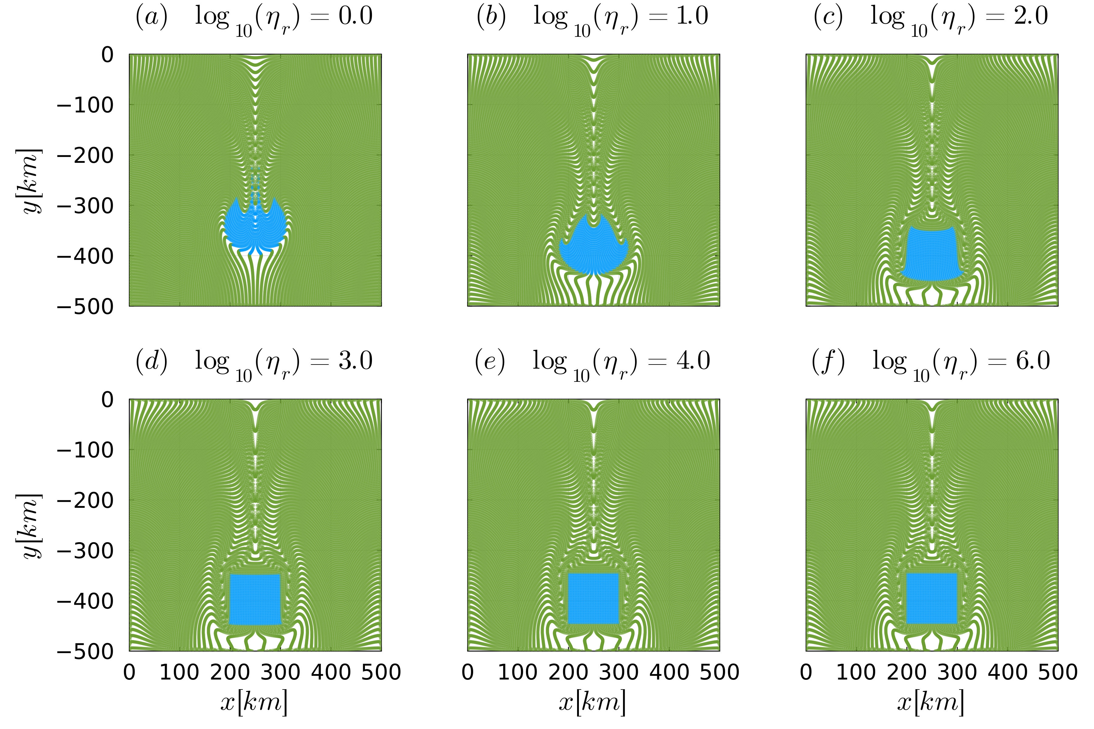
Figure 3. Final stage. Final stage of the sinking block for different viscosity ratios using the tracer method.