Rayleigh Taylor Instability (RTI)
This example demonstrates the transient behavior of a well-known problem in geodynamics: the Rayleigh–Taylor instability (RTI) in a two-layered system with different densities and viscosities. The script presents the setup and dynamic evolution of an RTI, which is also used in another script within GeoModBox.jl to benchmark the solution of the momentum equation under purely density-driven conditions.
The RTI model consists of two horizontally layered materials, each characterized by specified thickness, viscosity, and density. No-slip boundary conditions are applied at the top and bottom, and symmetric velocity boundary conditions at the lateral boundaries. If the interface between the layers is perturbed (e.g., sinusoidally), the system becomes unstable. The more buoyant lower layer rises while the denser upper layer sinks, with velocities increasing over time until a new stable configuration is reached.
The initial growth rate of the instability is mainly controlled by the density contrast, as well as the perturbation’s wavelength and amplitude. This can be estimated analytically. A benchmark example therefore is given in an additional script.
In the following, the focus lies on setting up the RTI instability using tracers, solving the momentum equation, and advecting the phase field.
Let's load the required modules first.
using Plots
using ExtendableSparse
using GeoModBox
using GeoModBox.InitialCondition, GeoModBox.MomentumEquation.TwoD
using GeoModBox.AdvectionEquation.TwoD
using GeoModBox.Tracers.TwoD
using Base.Threads
using Printf, LinearAlgebra
using TimerOutputs
To update the rheological information on the numerical grid, we first introduce a small helper function. The function is only required when the material properties are reconstructed from the interpolated phase ratio at the cell centroids. When direct marker interpolation is used, the density and viscosity fields are obtained directly from the marker distribution and this helper function is not needed. The helper function also computes the vertex viscosities required by the staggered-grid discretization.
function UpdateRheo(D,ρ,η,avg)

    # Density --- artihmetic averaging ---
    @. D.ρ     =   ρ[1]*(1.0 - D.p) + ρ[2]*D.p
    D.ρe[2:end-1,2:end-1]     .=  D.ρ
    D.ρe[1,:]     .=  D.ρe[2,:]
    D.ρe[end,:]   .=  D.ρe[end-1,:]
    D.ρe[:,1]     .=  D.ρe[:,2]
    D.ρe[:,end]   .=  D.ρe[:,end-1]

    # Viscosity - Centroids and vertices ---
    if avg ==     :arith
        @. D.ηc =   (1.0 - D.p) * η[1] + D.p * η[2]
    elseif avg == :harm
        @. D.ηc =   1.0 / ( (1.0 - D.p) / η[1] + D.p / η[2] )
    elseif avg == :geom
        @. D.ηc =   η[1]^(1.0 - D.p) * η[2]^D.p
    else
        error("Unknown viscosity averaging: $(avg)")
    end
    # --- Extended Centroids-
    D.ηce[2:end-1,2:end-1]     .=  D.ηc
    D.ηce[1,:]     .=  D.ηce[2,:]
    D.ηce[end,:]   .=  D.ηce[end-1,:]
    D.ηce[:,1]     .=  D.ηce[:,2]
    D.ηce[:,end]   .=  D.ηce[:,end-1]
    # --- Vertices -
    if avg == :arith
        @. D.ηv =
            0.25*(
                D.ηce[1:end-1,1:end-1] +
                D.ηce[2:end  ,1:end-1] +
                D.ηce[1:end-1,2:end  ] +
                D.ηce[2:end  ,2:end  ]
            )
    elseif avg == :harm
        @. D.ηv =
            4.0/(
                1/D.ηce[1:end-1,1:end-1] +
                1/D.ηce[2:end  ,1:end-1] +
                1/D.ηce[1:end-1,2:end  ] +
                1/D.ηce[2:end  ,2:end  ]
            )
    elseif avg == :geom
        @. D.ηv =
            exp(0.25*(
                log(D.ηce[1:end-1,1:end-1]) +
                log(D.ηce[2:end  ,1:end-1]) +
                log(D.ηce[1:end-1,2:end  ]) +
                log(D.ηce[2:end  ,2:end  ])
            ))
    else
        error("Unknown viscosity averaging: $(avg)")
    end

    return D
end
Next, we define the parameters controlling the initial phase distribution represented by the tracers. The material properties can be reconstructed on the numerical grid using two different approaches. In the first approach, the marker phases are bilinearly interpolated to the cell centers to obtain a phase ratio, from which the density and viscosity are reconstructed using a material mixing law. Alternatively, the density and viscosity stored on the markers can be transferred directly to the numerical grid using bilinear interpolation.
For this example, the direct marker interpolation together with arithmetic averaging is used. This combination provides a robust representation of the material interface for the large viscosity contrast considered here. The selected averaging scheme is applied consistently in both material-transfer strategies. For the phase-ratio approach it defines the material mixing law, whereas for direct marker interpolation it defines how marker properties are averaged during the transfer to the numerical grid. Alternative averaging schemes, such as geometric or harmonic averaging, are also available within GeoModBox.jl and may be explored by the user for comparison.
to          =   TimerOutput()
@timeit to "Ini" begin
save_fig    =   1
# How to update the numerical nodes from the marker ---
#   1) Phase ratio (:PhaseRatio), or
#   2) Direct bilinear interpolation of marker properties to the grid
#      (:MarkerInterpolation)
MaterialInterpolation   =   :MarkerInterpolation
# Define the averaging scheme used for both material-transfer methods:
#   1) Arithmetic   (:arith)
#   2) Geometric    (:geom)
#   3) Harmonic     (:harm)
avg                     =   :arith

MaterialInterpolation ∈ (:PhaseRatio, :MarkerInterpolation) ||
    error("Unknown material interpolation method: $MaterialInterpolation")
avg ∈ (:arith, :geom, :harm) ||
    error("Unknown averaging scheme: $avg")
# Although both strategies employ bilinear interpolation from the
# markers to the numerical grid, they differ in the quantity that is
# interpolated. The phase-ratio approach first interpolates the
# material phase and subsequently reconstructs the material
# properties using a mixing law, whereas the direct interpolation
# approach transfers the material properties themselves. Since
# viscosity is a nonlinear material property, the two approaches
# generally produce different numerical solutions.
# Define Initial Condition ========================================== #
Ini         =   (p=:RTI,)
λ           =   3.0e3           #   Perturbation wavelength[ m ]
δA          =   1500/15         #   Amplitude [ m ]
# ------------------------------------------------------------------- #
Note: "Viscosity averaging".
GeoModBox.jlprovides arithmetic, geometric, and harmonic averaging schemes for transferring viscosity information to the numerical grid. Arithmetic averaging is used as the default because it provides a robust representation of the material interface for the present example. The influence of alternative averaging schemes is beyond the scope of this introductory example but can be investigated by modifying the corresponding parameters.
The following parameters are used for visualization.
# Plot Settings ===================================================== #
Pl  =   (
    qinc    =   4,
    mainc   =   2,
    qsc     =   100*(60*60*24*365.25)*3
)
# ------------------------------------------------------------------- #
In the following the model geometry and the numerical gridding are defined. The aspect ratio and horizontal resolution of the model domain are defined by the wavelength of the perturbation.
# Geometry ========================================================== #
M       =   Geometry(
    ymin    =   -3.0e3,     # [ m ]
    ymax    =   0.0,
    xmin    =   0.0,
)
ar          =   Int64(2 * λ / (M.ymax-M.ymin))  #   aspect ratio
M.xmax      =   (M.ymax-M.ymin)*ar
# -------------------------------------------------------------------- #
# Grid =============================================================== #
NC  =   (
    x   =   50*ar,
    y   =   50,
)
NV  =   (
    x   =   NC.x + 1,
    y   =   NC.y + 1,
)
Δ       =   GridSpacing(
    x   =   (M.xmax - M.xmin)/NC.x,
    y   =   (M.ymax - M.ymin)/NC.y,
)
x       =   (
    c   =   LinRange(M.xmin+Δ.x/2,M.xmax-Δ.x/2,NC.x),
    ce  =   LinRange(M.xmin - Δ.x/2.0, M.xmax + Δ.x/2.0, NC.x+2),
    v   =   LinRange(M.xmin,M.xmax,NV.x),
)
y       =   (
    c   =   LinRange(M.ymin+Δ.y/2,M.ymax-Δ.y/2,NC.y),
    ce  =   LinRange(M.ymin - Δ.y/2.0, M.ymax + Δ.y/2.0, NC.y+2),
    v   =   LinRange(M.ymin,M.ymax,NV.y),
)
x1      =   (
    c2d     =   x.c .+ 0*y.c',
    v2d     =   x.v .+ 0*y.v',
    vx2d    =   x.v .+ 0*y.ce',
    vy2d    =   x.ce .+ 0*y.v',
)
x   =   merge(x,x1)
y1      =   (
    c2d     =   0*x.c .+ y.c',
    v2d     =   0*x.v .+ y.v',
    vx2d    =   0*x.v .+ y.ce',
    vy2d    =   0*x.ce .+ y.v',
)
y   =   merge(y,y1)
# -------------------------------------------------------------------- #
Next, define the physical parameters for the two layers.
# Physics ============================================================ #
g       =   10.0                #   Gravitational acceleration [ m/s^2 ]
# 0 - upper layer; 1 - lower layer
η₀      =   1e19                #   Viscosity composition 0 [ Pa s ]
η₁      =   1e13                #   Viscosity composition 1 [ Pa s]
ηᵣ      =   log10(η₁/η₀)
η       =   [η₀,η₁]             #   Viscosity for phases

ρ₀      =   3000.0              #   Density composition 0 [ kg/m^3 ]
ρ₁      =   2900.0              #   Density composition 1 [ kg/m^3 ]
ρ       =   [ρ₀,ρ₁]             #   Density for phases

phase   =   [0,1]
# -------------------------------------------------------------------- #
For visualization purposes, a filename for the GIF animation must be defined.
# Animation and Plot Settings ======================================= #
path        =   string("./examples/StokesEquation/2D/Results/")
anim        =   Plots.Animation(path, String[] )
filename    =   string(Ini.p,"_ηr_",round(ηᵣ),
                        "_tracers_DC_",MaterialInterpolation,"_",
                        avg)
# ------------------------------------------------------------------- #
Since the energy equation is not solved, fewer data fields need to be initialized. The momentum equation is solved using the defect correction method. Therefore the strain rate and stress components are requirerd as well.
# Allocation ======================================================== #
D       =   (
    ρ       =   zeros(Float64,(NC...)),
    ρe      =   zeros(Float64,(NC.x+2,NC.y+2)),
    cp      =   zeros(Float64,(NC...)),
    vx      =   zeros(Float64,(NV.x,NV.y+1)),
    vy      =   zeros(Float64,(NV.x+1,NV.y)),
    Pt      =   zeros(Float64,(NC...)),
    vxc     =   zeros(Float64,(NC...)),
    vyc     =   zeros(Float64,(NC...)),
    vc      =   zeros(Float64,(NC...)),
    wt      =   zeros(Float64,(NC.x,NC.y)),
    wte     =   zeros(Float64,(NC.x+2,NC.y+2)),
    wtv     =   zeros(Float64,(NV.x,NV.y)),
    ηc      =   zeros(Float64,NC...),
    ηce     =   zeros(Float64,(NC.x+2,NC.y+2)),
    ηv      =   zeros(Float64,NV...),
    p       =   zeros(Float64,NC...),
    p_ex    =   zeros(Float64,(NC.x+2,NC.y+2)),
)
# ------------------------------------------------------------------- #
# Needed for the defect correction solution ---
divV        =   zeros(Float64,NC...)
ε           =   (
    xx      =   zeros(Float64,NC...),
    yy      =   zeros(Float64,NC...),
    xy      =   zeros(Float64,NV...),
)
τ           =   (
    xx      =   zeros(Float64,NC...),
    yy      =   zeros(Float64,NC...),
    xy      =   zeros(Float64,NV...),
)
# ------------------------------------------------------------------- #
No-slip velocity boundary conditions are applied at the top and bottom, and free-slip conditions along the lateral boundaries.
# Boundary Conditions =============================================== #
VBC     =   (
    type    =   (E=:freeslip,W=:freeslip,S=:noslip,N=:noslip),
    val     =   (E=zeros(NV.y),W=zeros(NV.y),S=zeros(NV.x),N=zeros(NV.x),
                    vyS=0.0,vyN=0.0,vxW=0.0,vxE=0.0),
)
# ------------------------------------------------------------------- #
The number of time steps is arbitrarily limited to a maximum of 50 iterations. This enables the rise of multiple dikes without reaching a full overturn of the system.
# Time ============================================================== #
T   =   TimeParameter(
    tmax    =   10.0,           #   [ Ma ]
    Δfacc   =   1.0,            #   Courant time factor
    itmax   =   200,            #   Maximum iterations; 50
)
T.tmax      =   T.tmax*1e6*T.year    #   [ s ]
T.Δ         =   T.Δfacc * minimum((Δ.x,Δ.y)) /
                    (sqrt(maximum(abs.(D.vx))^2 + maximum(abs.(D.vy))^2))

Time        =   zeros(T.itmax)
final_step  =   0
# ------------------------------------------------------------------- #
In the following the tracers are initialized.
# Tracer Advection ================================================== #
@timeit to "Tracer Ini" begin
nmx,nmy     =   5,5
noise       =   0
nmark       =   nmx*nmy*NC.x*NC.y
Aparam      =   :phase
MPC         =   (
        c       =   zeros(Float64,(NC.x,NC.y)),
        v       =   zeros(Float64,(NV.x,NV.y)),
        th      =   zeros(Float64,(nthreads(),NC.x,NC.y)),
        thv     =   zeros(Float64,(nthreads(),NV.x,NV.y)),
)
MAVG        = (
        PC_th   =   [similar(D.wte) for _ = 1:nthreads()],  # per thread
        PV_th   =   [similar(D.wtv) for _ = 1:nthreads()],   # per thread
        wte_th  =   [similar(D.wte) for _ = 1:nthreads()],  # per thread
        wtv_th  =   [similar(D.wtv) for _ = 1:nthreads()],  # per thread
)
Ma      =   IniTracer2D(Aparam,nmx,nmy,Δ,M,NC,noise,Ini.p,phase;λ,δA)
# RK4 weights ---
rkw     =   1.0/6.0*[1.0 2.0 2.0 1.0]   # for averaging
rkv     =   1.0/2.0*[1.0 1.0 2.0 2.0]   # for time stepping
# Count marker per cell ---
CountMPC(Ma,nmark,MPC,M,x,y,Δ,NC,NV)
if MaterialInterpolation == :PhaseRatio
    # Phase ---
    Markers2Cells(Ma,nmark,MAVG.PC_th,D.p_ex,MAVG.wte_th,D.wte,x,y,Δ,Aparam,phase)
    D.p     .=  D.p_ex[2:end-1,2:end-1]
    UpdateRheo(D,ρ,η,avg)
elseif MaterialInterpolation == :MarkerInterpolation
    # Interpolate from markers to cell ---
    Markers2Cells(Ma,nmark,MAVG.PC_th,D.p_ex,MAVG.wte_th,D.wte,x,y,Δ,Aparam,phase)
    D.p     .=  D.p_ex[2:end-1,2:end-1]
    Markers2Cells(Ma,nmark,MAVG.PC_th,D.ρe,MAVG.wte_th,D.wte,x,y,Δ,Aparam,ρ)
    D.ρ     .=   D.ρe[2:end-1,2:end-1]
    Markers2Cells(Ma,nmark,MAVG.PC_th,D.ηce,MAVG.wte_th,D.wte,x,y,Δ,Aparam,η;avgm=avg)
    D.ηc    .=   D.ηce[2:end-1,2:end-1]
    Markers2Vertices(Ma,nmark,MAVG.PV_th,D.ηv,MAVG.wtv_th,D.wtv,x,y,Δ,Aparam,η;avgm=avg)
else
    error("Unknown material interpolation method: $MaterialInterpolation")
end
end
# ------------------------------------------------------------------- #
To solve the linear system of equations, one needs to defined the numbering of the unknowns and initialize the residual and the correction term arrays.
# System of Equations =============================================== #
# Iterations
niter   =   50
ϵ       =   1e-10
# Numbering, without ghost nodes! ---
off    = [  NV.x*NC.y,                          # vx
            NV.x*NC.y + NC.x*NV.y,              # vy
            NV.x*NC.y + NC.x*NV.y + NC.x*NC.y]  # Pt

Num    =    (
    Vx  =   reshape(1:NV.x*NC.y, NV.x, NC.y),
    Vy  =   reshape(off[1]+1:off[1]+NC.x*NV.y, NC.x, NV.y),
    Pt  =   reshape(off[2]+1:off[2]+NC.x*NC.y,NC...),
            )
δx      =   zeros(maximum(Num.Pt))
F       =   zeros(maximum(Num.Pt))
# Residuals ---
Fm     =    (
    x       =   zeros(Float64,NV.x, NC.y),
    y       =   zeros(Float64,NC.x, NV.y)
)
FPt     =   zeros(Float64,NC...)
# ------------------------------------------------------------------- #
end
Now, the time loop can be started.
# Time Loop ========================================================= #
@timeit to "Time Loop" begin
for it = 1:T.itmax
    # Update Time ---
    if it > 1
        Time[it]   =   Time[it-1] + T.Δ
    end
    @printf("Time step: #%04d, Time [Myr]: %04e\n ",it,
                Time[it]/(60*60*24*365.25)/1.0e6)
An initial guess is provided for the momentum equation, and residuals are computed iteratively. Within the defect correction method, the coefficient matrix is assembled to calculate the correction term for the initial guess.
    @printf("---Momentum Calculation ---\n")
    # Momentum Equation ===
    # Initial Residual ---------------------------------------------- #
    D.vx    .=  0.0
    D.vy    .=  0.0
    D.Pt    .=  1.0
    @timeit to "Solution Iteration" begin
    # Assemble Coefficients ========================================= #
    @timeit to "Assembly" begin
    K       =   Assembly(NC, NV, Δ, D.ηc, D.ηv, VBC, Num)
    Kfac    =   lu(K.cscmatrix)
    end
    for iter=1:niter
        @timeit to "Residual" begin
        Residuals2D!(D,VBC,ε,τ,divV,Δ,D.ηc,D.ηv,g,Fm,FPt)
        F[Num.Vx]   .=   Fm.x
        F[Num.Vy]   .=   Fm.y
        F[Num.Pt]   .=   FPt
        @printf("||R|| = %1.4e\n", norm(F)/length(F))
        norm(F)/length(F) < ϵ ? break : nothing
        end
        # --------------------------------------------------------------- #
        # Solution of the linear system ================================= #
        @timeit to "Solution" begin
        δx      =   - (Kfac \ F)
        end
        # --------------------------------------------------------------- #
        # Update Unknown Variables ====================================== #
        D.vx[:,2:end-1]     .+=  δx[Num.Vx]
        D.vy[2:end-1,:]     .+=  δx[Num.Vy]
        D.Pt                .+=  δx[Num.Pt]
    end
    end
    # --------------------------------------------------------------- #
For visualization, the centroid velocity field is computed. The density, marker distribution, absolut velocity and centroid viscosity is plotted for certain time steps. Depending on the parameter save_fig the plot is displayed or stored to generate a gif animation.
    # Get the velocity on the centroids ---
    for i = 1:NC.x
        for j = 1:NC.y
            D.vxc[i,j]  = (D.vx[i,j+1] + D.vx[i+1,j+1])/2
            D.vyc[i,j]  = (D.vy[i+1,j] + D.vy[i+1,j+1])/2
        end
    end
    @. D.vc        = sqrt(D.vxc^2 + D.vyc^2)
    # ---
    if mod(it,5) == 0 || final_step == 1 || it == 1
        p = heatmap(x.c./1e3,y.c./1e3,D.ρ',color=:inferno,
                    xlabel="x[km]",ylabel="y[km]",colorbar=true,
                    title="ρ",
                    aspect_ratio=:equal,xlims=(M.xmin/1e3, M.xmax/1e3),
                    ylims=(M.ymin/1e3, M.ymax/1e3),
                    layout=(2,2),subplot=1)
        scatter!(p,Ma.x[1:Pl.mainc:end]./1e3,Ma.y[1:Pl.mainc:end]./1e3,
                    ms=1,ma=0.5,mc=Ma.phase[1:Pl.mainc:end],markerstrokewidth=0.0,
                    xlabel="x[km]",ylabel="y[km]",colorbar=true,
                    title="tracers",label="",
                    aspect_ratio=:equal,xlims=(M.xmin/1e3, M.xmax/1e3),
                    ylims=(M.ymin/1e3, M.ymax/1e3),
                    layout=(2,2),subplot=2)
        heatmap!(p,x.c./1e3,y.c./1e3,D.vc',
                    xlabel="x[km]",ylabel="y[km]",colorbar=true,
                    title="V_c",color=cgrad(:batlow),
                    aspect_ratio=:equal,xlims=(M.xmin/1e3, M.xmax/1e3),
                    ylims=(M.ymin/1e3, M.ymax/1e3),
                    layout=(2,2),subplot=4)
        quiver!(p,x.c2d[1:Pl.qinc:end,1:Pl.qinc:end]./1e3,
                    y.c2d[1:Pl.qinc:end,1:Pl.qinc:end]./1e3,
                    quiver=(D.vxc[1:Pl.qinc:end,1:Pl.qinc:end].*Pl.qsc,
                            D.vyc[1:Pl.qinc:end,1:Pl.qinc:end].*Pl.qsc),
                    la=0.5,color="white",layout=(2,2),subplot=4)
        heatmap!(p,x.c./1e3,y.c./1e3,log10.(D.ηc'),color=reverse(cgrad(:roma)),
                    xlabel="x[km]",ylabel="y[km]",title="η_c",
                    clims=extrema(log10.(η)),
                    aspect_ratio=:equal,xlims=(M.xmin/1e3, M.xmax/1e3),
                    ylims=(M.ymin/1e3, M.ymax/1e3),colorbar=true,
                    layout=(2,2),subplot=3)
        if save_fig == 1
            Plots.frame(anim)
        elseif save_fig == 0
            display(p)
        end
    end
    if final_step == 1
        @printf(" Maximum Time reached!\n")
        break
    end
Since only the momentum and mass conservation equations are solved, the maximum time step is fully governed by the Courant criterium.
    # Calculate Time Stepping ---
    T.Δ        =   T.Δfacc * minimum((Δ.x,Δ.y)) /
            (sqrt(maximum(abs.(D.vx))^2 + maximum(abs.(D.vy))^2))
    if Time[it] >= T.tmax
        T.Δ         =   T.tmax - Time[it-1]
        Time[it]    =   Time[it-1] + T.Δ
        final_step  =   1
    end
Now, one can advect the phases on the tracers using the staggered velocity field and Runge-Kutta 4th order. Following the advection, the information on the centroids and vertices is updated from the markers.
    # Advection ===
    @timeit to "Tracer Advection" begin
    # Advect tracers ---
    @printf("Running on %d thread(s)\n", nthreads())
    AdvectTracer2D(Ma,nmark,D,x,y,T.Δ,Δ,NC,rkw,rkv)
    CountMPC(Ma,nmark,MPC,M,x,y,Δ,NC,NV)
    if MaterialInterpolation == :PhaseRatio
        # Phase ---
        Markers2Cells(Ma,nmark,MAVG.PC_th,D.p_ex,MAVG.wte_th,D.wte,x,y,Δ,Aparam,phase)
        D.p     .=  D.p_ex[2:end-1,2:end-1]
        UpdateRheo(D,ρ,η,avg)
    elseif MaterialInterpolation == :MarkerInterpolation
        # Interpolate phase from tracers to grid ---
        Markers2Cells(Ma,nmark,MAVG.PC_th,D.p_ex,MAVG.wte_th,D.wte,x,y,Δ,Aparam,phase)
        D.p     .=  D.p_ex[2:end-1,2:end-1]
        Markers2Cells(Ma,nmark,MAVG.PC_th,D.ρe,MAVG.wte_th,D.wte,x,y,Δ,Aparam,ρ)
        D.ρ     .=   D.ρe[2:end-1,2:end-1]
        Markers2Cells(Ma,nmark,MAVG.PC_th,D.ηce,MAVG.wte_th,D.wte,x,y,Δ,Aparam,η;avgm=avg)
        D.ηc    .=   D.ηce[2:end-1,2:end-1]
        Markers2Vertices(Ma,nmark,MAVG.PV_th,D.ηv,MAVG.wtv_th,D.wtv,x,y,Δ,Aparam,η;avgm=avg)
    else
        error("Unknown material interpolation method: $MaterialInterpolation")
    end
    end
    @printf("\n")
end # End Time Loop
end
Finally, the gif animation is generated.
if save_fig == 1
    # Write the frames to a GIF file
    Plots.gif(anim, string( path, filename, ".gif" ), fps = 15)
    foreach(rm, filter(startswith(string(path,"00")), readdir(path,join=true)))
end
display(to)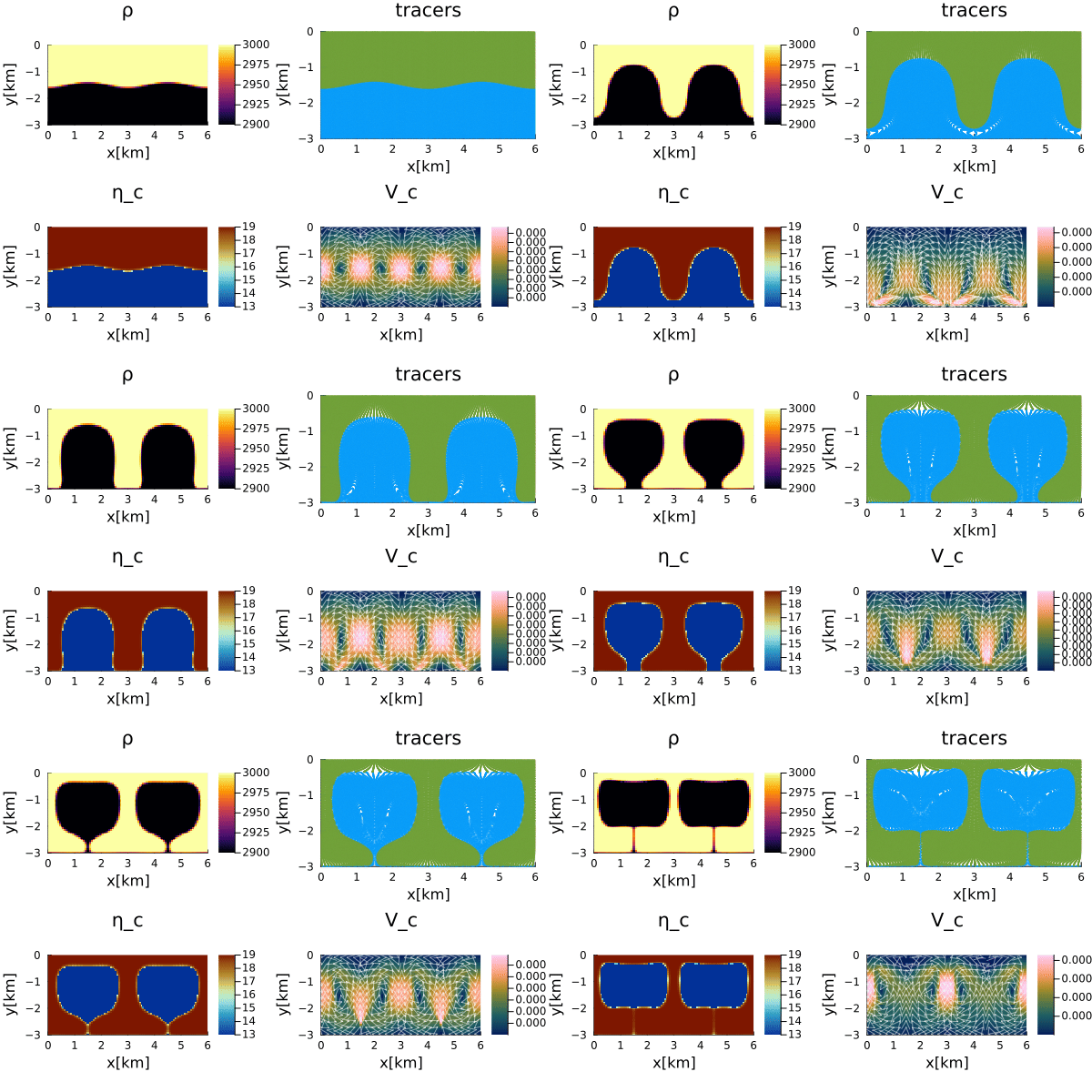
Figure 1. Rayleigh–Taylor Instability. Transient evolution of a two-layer system with a density contrast of 100 kg/m³ and a viscosity contrast spanning six orders of magnitude. Density is reconstructed from the phase ratio for the PhaseRatio approach. Panels show: density (top left), tracer distribution (top right), centroid viscosity (bottom left), and absolute centroid velocity (bottom right).