Stokes Equation (2D)

For creeping flows, the conservation of momentum reduces to the Stokes equations,

\[\begin{equation} 0 = -\frac{\partial{P}}{\partial{x_i}} + \frac{\partial{\tau_{ij}}}{\partial{x_j}} + \rho g_i, \end{equation}\]

where $P$ is the pressure [Pa], $\rho$ is the density [kg/m³], $g_i$ is the gravitational acceleration [m/s²], $\frac{\partial}{\partial x_i}$ is the spatial derivative in the $x_i$-direction, and $\tau_{ij}$ is the deviatoric stress tensor [Pa], defined as:

\[\begin{equation} \tau_{ij} = 2\eta \dot{\varepsilon}_{ij}, \end{equation}\]

where $\eta$ is the viscosity [Pa·s], and $\dot{\varepsilon}_{ij}$ is the strain-rate tensor [1/s], given by:

\[\begin{equation} \dot{\varepsilon}_{ij} = \frac{1}{2} \left( \frac{\partial{v_i}}{\partial{x_j}} + \frac{\partial{v_j}}{\partial{x_i}} \right), \end{equation}\]

where $v_i$ is the velocity [m/s] in the $i$-th direction.

The Stokes equation yields two equations for the three unknowns $v_x$, $v_y$, and $P$. An additional equation is therefore required: the mass conservation equation.

The conservation of mass is described in the Eulerian reference frame by

\[\begin{equation} \frac{\partial{\rho}}{\partial{t}} + \frac{\partial}{\partial{x_i}}\left(\rho v_i\right)=0, \end{equation}\]

which describes the conservation of mass within an infinitesimal control volume. The first term represents the temporal change in mass within the control volume, whereas the second term represents the net mass flux across its boundaries. Applying the product rule to the second term of Equation (4), together with the definition of the material derivative, yields the Lagrangian form of the mass conservation equation

\[\begin{equation} \frac{1}{\rho}\frac{D \rho}{D t}+\frac{\partial{v_i}}{\partial{x_i}}=0 \end{equation}\]

Assuming an incompressible fluid $\left(\frac{D \rho}{D t} \equiv 0 \right)$, Equation (5) simplifies to the continuity equation

\[\begin{equation} \frac{\partial{v_i}}{\partial{x_i}} = 0. \end{equation}\]

Together, the Stokes and continuity equations form a closed system for the unknown velocity and pressure variables.

Discretization

To numerically solve Equations (1) and (6), the spatial domain must be discretized and the relevant properties assigned to the appropriate computational nodes. Thus, the equations are discretized on a staggered finite difference grid, where the horizontal (cyan dashes) and vertical (orange dashes) velocities are defined between the regular grid points (vertices), and the pressure (red circles) within finite difference cells (centroids), as shown in Figure 1.

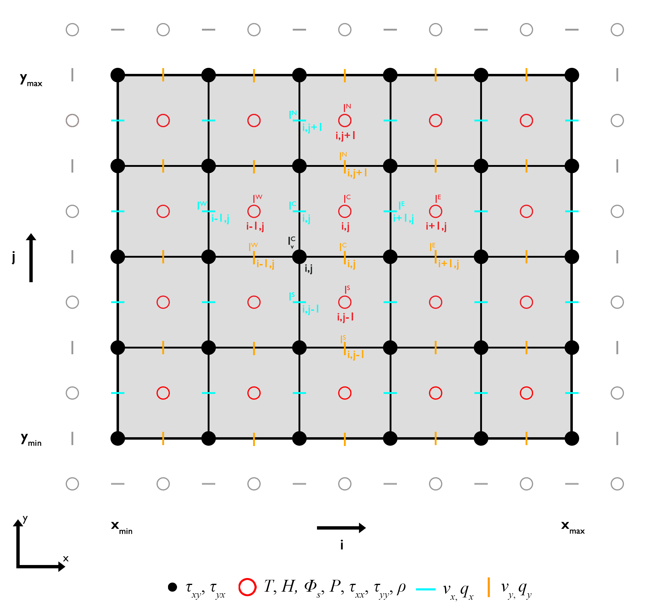
Figure 1. Staggered finite difference grid for the momentum and mass conservation equation. The horizontal and vertical velocities require ghost nodes at the North, South, East, and West boundaries, respectively.

A staggered grid enables conservation of stress between adjacent grid points and requires careful placement of the associated variables. Each equation is evaluated at the central node of its respective variable grid, requiring values from neighboring nodes defined by the numerical stencil. The locations of these points in a finite difference scheme are determined by a numerical stencil. Thus, care needs to be taken generating the index for the variables. For the 2D Stokes equation in combination with the 2D mass conservation equation, different numerical stencils need to be considered, especially for cases of constant and variable viscosity. The stencils for each equation assuming constant or variable viscosity are discussed in more detail below. The spatial discretization relies on central finite differences to approximate both the velocity and pressure gradients.

The indices of the adjacent points, which determine the positions of the coefficients in the coefficient matrix, can be expressed using the local indices $i$ and $j$ of each numerical grid. Because a staggered grid is used, each variable field ($v_x$, $v_y$, $P$, $\tau_{ij}$, $\eta$, and $\rho$) is defined on its own grid and therefore possesses its own local indices $(i,j)$ and a variable-specific global index. The local indices describe the position of the computational node of each corresponding variable grid in the horizontal and vertical directions, respectively. The global index assumes a horizontal numbering through the model domain; that is, the numbering proceeds row by row from the bottom to the top. The indices for the adjacent centroid points follows the indexing convention described in the general solution section.

For clarity, two types of global indices are used below:

• variable-specific global indices, which number the nodes of a single grid (e.g. centroids or vertices),
• system global indices, which number the unknowns in the assembled linear system.

The variable-specific global index indicates the position relative to the central reference point (e.g., $N$, $S$).

The global index for density, for example, is defined by consecutively numbering the centroids:

\[\begin{equation} I^\textrm{C}_c = \left(j-1\right) nc_x + i, \end{equation}\]

where $nc_x$ is the total number of centroids in the horizontal direction. Here, it is important to distinguish between the centroid index used for density and the system global index used for pressure, because pressure is part of the consecutively numbered unknowns in the assembled system of equations (see below).

The global index for the shear stress, for example, is defined by consecutively numbering the vertices:

\[\begin{equation} I^\textrm{C}_v = \left(j-1\right) nv_x + i, \end{equation}\]

where $nv_x$ is the total number of vertices in the horizontal direction.

The global indexing for the unknown variables in the system of equations proceeds by:

1. Enumerating all equations for the $x$-component of momentum (unknown $v_x$),

2. Followed by the $y$-component of momentum (unknown $v_y$),

3. And finally the mass conservation equation (unknown $P$).

The numbering $I$ for each equation is then defined as:

$x$-component ($v_x$)

\[\begin{equation} I^\textrm{C}_{x} = 1 : \left(nv_x \cdot nc_y\right), \end{equation}\]

$y$-component ($v_y$)

\[\begin{equation} I^\textrm{C}_{y} = \left(nv_x \cdot nc_y + 1 \right) : \left(nv_x \cdot nc_y + nc_x \cdot nv_y\right), \end{equation}\]

Mass Conservation ($P$)

\[\begin{equation} I^\textrm{C}_{p} = \left(nv_x \cdot nc_y + nc_x \cdot nv_y + 1\right) : \left(nv_x \cdot nc_y + nc_x \cdot nv_y + nc_x \cdot nc_y\right). \end{equation}\]

This results in a consecutive global numbering of the system of equations for the $x$- and $y$-component of the momentum and the mass conservation equation. Each discretized equation corresponds to a row $I^\textrm{C}_{x,y,p}$ in the coefficient matrix.

Note: The index $I^\textrm{C}_{x,y,p}$ for the system of equations is not the same as the consecutive numbering of the velocity and pressure nodes $I^\textrm{C}$, which only considers the global numbering for one single variable.

The nonzero entries within a given matrix row appear at column positions corresponding to the neighboring variables involved in the stencil. These column indices are denoted by $I^k_{x,y,mc}$, where $k \in \{\textrm{S}, \textrm{SW}, \textrm{SE}, \textrm{W}, \textrm{C}, \textrm{E}, \textrm{NW}, \textrm{NE}, \textrm{N}\}$. The column index of each coefficient is computed relative to the central row index $I^\textrm{C}_{x,y,p}$. Thereby, the coefficient indices slightly vary for constant and variable viscosity cases. Note that cross terms involving $v_y$ and $v_x$ are indexed using the $y$- and $x$-component system indices, reflecting the staggered grid arrangement.

Constant Viscosity

$x$-component

\[\begin{equation}\begin{split} I^\textrm{S}_{x} & = I^\textrm{C}_{x} - nv_x, \\ I^\textrm{W}_{x} & = I^\textrm{C}_{x} - 1, \\ I^\textrm{E}_{x} & = I^\textrm{C}_{x} + 1, \\ I^\textrm{N}_{x} & = I^\textrm{C}_{x} + nv_x, \end{split}\end{equation}\]

and for the pressure gradient

\[\begin{equation} I^\textrm{W}_p = I^\textrm{C}_p - 1. \end{equation}\]

$y$-component

\[\begin{equation}\begin{split} I^\textrm{S}_{y} & = I^\textrm{C}_{y} - nc_x, \\ I^\textrm{W}_{y} & = I^\textrm{C}_{y} - 1, \\ I^\textrm{E}_{y} & = I^\textrm{C}_{y} + 1, \\ I^\textrm{N}_{y} & = I^\textrm{C}_{y} + nc_x, \end{split}\end{equation}\]

and for the pressure gradient

\[\begin{equation} I^\textrm{S}_p = I^\textrm{C}_p - nc_x. \end{equation}\]

Variable Viscosity

$x$-component

\[\begin{equation}\begin{split} I^\textrm{S}_{x} & = I^\textrm{C}_{x} - nv_x, \\ I^\textrm{SW}_{x} & = I^\textrm{C}_{y} - 1, \\ I^\textrm{SE}_{x} & = I^\textrm{C}_{y}, \\ I^\textrm{W}_{x} & = I^\textrm{C}_{x} - 1, \\ I^\textrm{E}_{x} & = I^\textrm{C}_{x} + 1, \\ I^\textrm{NW}_{x} & = I^\textrm{C}_{y} + nc_x, \\ I^\textrm{NE}_{x} & = I^\textrm{C}_{y} + nc_x + 1, \\ I^\textrm{N}_{x} & = I^\textrm{C}_{x} + nv_x, \end{split}\end{equation}\]

and for the pressure gradient

\[\begin{equation} I^\textrm{W}_p = I^\textrm{C}_p - 1. \end{equation}\]

$y$-component

\[\begin{equation}\begin{split} I^\textrm{S}_{y} & = I^\textrm{C}_{y} - nc_x, \\ I^\textrm{SW}_{y} & = I^\textrm{C}_{x} - nv_x, \\ I^\textrm{SE}_{y} & = I^\textrm{C}_{x} - nv_x + 1, \\ I^\textrm{W}_{y} & = I^\textrm{C}_{y} - 1, \\ I^\textrm{E}_{y} & = I^\textrm{C}_{y} + 1, \\ I^\textrm{NW}_{y} & = I^\textrm{C}_{x}, \\ I^\textrm{NE}_{y} & = I^\textrm{C}_{x} + 1, \\ I^\textrm{N}_{y} & = I^\textrm{C}_{y} + nc_x, \end{split}\end{equation}\]

and for the pressure gradient

\[\begin{equation} I^\textrm{S}_p = I^\textrm{C}_p - nc_x. \end{equation}\]

The coefficients for the conservation of mass remain the same independent of the state of the viscosity.

Mass Conservation (mc)

\[\begin{equation}\begin{split} I^\textrm{S}_{mc} & = I^\textrm{C}_{y}, \\ I^\textrm{W}_{mc} & = I^\textrm{C}_{x}, \\ I^\textrm{C}_{mc} & = I^\textrm{C}_{p}, \\ I^\textrm{E}_{mc} & = I^\textrm{E}_{x}, \\ I^\textrm{N}_{mc} & = I^\textrm{N}_{y}. \end{split}\end{equation}\]

Field Management

For solving the incompressible Stokes equations in GeoModBox.jl, a staggered grid is employed. Velocity ghost nodes are introduced for the horizontal velocity component at the North and South boundaries and for the vertical velocity component at the East and West boundaries of the model domain. Consequently, each velocity field is extended in the direction normal to the boundary on which no velocity nodes are located.

The momentum residual is evaluated only at interior velocity nodes, whereas the continuity residual is evaluated at cell centers. Velocity values located on the domain boundaries are prescribed by the selected boundary conditions (e.g., no-slip, free-slip, constant velocity, or pure shear) and therefore do not constitute unknowns of the momentum equations. Instead, the corresponding rows of the linear system enforce the prescribed boundary values directly. For velocity nodes adjacent to the boundaries, ghost-node values are constructed from the boundary conditions and are used to evaluate the stress divergence appearing in the momentum residual.

Within GeoModBox.jl, the residual is calculated separately for each 2D variable field using the corresponding local indices. The momentum and continuity residuals are first evaluated on their native staggered grids and are subsequently assembled into a single one-dimensional residual vector using the global indexing defined in Equations (9)–(11). The size of the linear system is determined by the total number of degrees of freedom. The coefficients of the matrix are modified directly according to the prescribed boundary conditions. During the defect-correction iteration, the computed correction vector is added to the current solution estimate. Both the correction vector and the solution vector store the unknowns $v_x$, $v_y$, and $P$ in the one-dimensional ordering introduced above. In the following, the global index always refers to this total 1D vector.

For the direct solution strategy based on a single left-matrix division, the same coefficient matrix is assembled. Instead of evaluating a residual, the boundary-condition contributions are incorporated into the right-hand side of the linear system, which is then solved directly.

Boundary Conditions

To impose boundary conditions on the staggered velocity grid, ghost nodes located a distance $\frac{\Delta x}{2}$ and $\frac{\Delta y}{2}$ outside the computational domain are introduced. However, ghost nodes for the velocities are only required in the direction where the corresponding velocity component is located at a cell face rather than directly on the boundary (see Figure 1). The velocity values at these ghost nodes are directly included in the discretized FD formulations for the nodes adjacent to the boundaries.

GeoModBox.jl supports four boundary-condition types for the momentum equations: free-slip, no-slip, constant velocity, and pure shear. These correspond to different combinations of Dirichlet and Neumann conditions imposed on the normal and tangential velocity components.

Constant-velocity boundary conditions are implemented analogously to the no-slip condition, except that the prescribed boundary velocity may take an arbitrary constant value. For pure-shear boundary conditions, the normal velocity component is prescribed at the corresponding boundary, while the tangential velocity satisfies a zero normal derivative, analogous to the free-slip condition.

For boundaries requiring ghost nodes, the ghost-node values are chosen such that linear interpolation between the ghost node and the adjacent interior node recovers the prescribed boundary velocity (e.g., $v_{x,S}$, $v_{x,N}$, $v_{y,E}$, and $v_{y,W}$). Consequently, all velocity components must be specified when prescribing a deformation field such as pure shear.

In the following, the ghost-node values are obtained by enforcing either a zero normal derivative (free-slip) or a prescribed boundary velocity (no-slip or constant velocity) using linear interpolation between the ghost node and the adjacent interior node.

Free-slip

Free-slip boundary conditions allow fluid motion along the boundary while enforcing zero shear stress and no flow across the boundary. For the lateral boundaries (East, West), this translates to:

\[\begin{equation} \begin{split} v_x = 0, \\ \frac{\partial{v_{y}}}{\partial{x}}=0. \end{split} \end{equation}\]

For the horizontal boundaries (North, South), the conditions are:

\[\begin{equation} \begin{split} v_y = 0, \\ \frac{\partial{v_{x}}}{\partial{y}}=0. \end{split} \end{equation}\]

$x$-component

For the free-slip condition, the horizontal velocity $v_x$ at the ghost nodes along the South and North boundaries is then defined as

South

\[\begin{equation} v_{x,G^S} = v_{x,(:,1)}, \end{equation}\]

North

\[\begin{equation} v_{x,G^N} = v_{x,(:,nc_y)}. \end{equation}\]

Since the horizontal velocity nodes lie directly on the East and West boundaries, the normal velocity is prescribed directly as $v_x = 0$.

$y$-component

The vertical velocity $v_y$ at the ghost nodes for the West and East boundaries is defined as:

West

\[\begin{equation} v_{y,G^W} = v_{y,(1,:)}, \end{equation}\]

East

\[\begin{equation} v_{y,G^E} = v_{y,(nc_x,:)}. \end{equation}\]

Since the vertical velocity nodes lie directly on the North and South boundaries, the normal velocity is prescribed directly as $v_y = 0$.

No-slip

No-slip boundary conditions enforce zero velocity relative to the boundary. Thus, for all boundaries (East, West, South, and North), the velocity components satisfy:

\[\begin{equation} \begin{split} v_x = 0, \\ v_y = 0. \end{split} \end{equation}\]

$x$-component

For the horizontal velocity $v_x$, values at the ghost nodes adjacent to the South and North boundaries are defined as:

South

\[\begin{equation} v_{x,G^S} = 2V_{BC}^S - v_{x,(:,1)}, \end{equation}\]

North

\[\begin{equation} v_{x,G^N} = 2V_{BC}^N - v_{x,(:,nc_y)}, \end{equation}\]

where $V_{BC}^S$ and $V_{BC}^N$ are the prescribed boundary velocities (typically zero for no-slip).

At the lateral boundaries (East, West), the velocity nodes fall directly on the boundary and thus, $v_x$ is set to zero, as in the free-slip case.

$y$-component

For the vertical velocity $v_y$, the ghost nodes adjacent to the West and East boundaries are defined as:

West

\[\begin{equation} v_{y,G^W} = 2V_{BC}^W - v_{y,(1,:)}, \end{equation}\]

East

\[\begin{equation} v_{y,G^E} = 2V_{BC}^E - v_{y,(nc_x,:)}, \end{equation}\]

where $V_{BC}^W$ and $V_{BC}^E$ are the prescribed boundary velocities (again typically zero).

Along the North and South boundaries, the velocity nodes fall directly on the boundary and thus, $v_y$ is set to zero, consistent with the free-slip implementation.

Constant velocity

Constant-velocity boundary conditions prescribe both velocity components at the boundary. On a staggered grid, the velocity component located directly on the boundary is prescribed explicitly, whereas the complementary velocity component is imposed through a ghost-node formulation such that its linearly interpolated value at the boundary equals the prescribed velocity. The implementation is therefore identical to the no-slip condition, except that the prescribed boundary velocity may take any constant value.

For example, on the West boundary the horizontal velocity is prescribed directly at the boundary node and the vertical velocity is prescribed through the ghost node,

\[\begin{equation} v_{x,(1,:)} = V_{BC}^W, \end{equation}\]

\[\begin{equation} v_{y,G^W} = 2V_{BC}^W - v_{y,(1,:)}, \end{equation}\]

analogously, on the South boundary

\[\begin{equation} v_{x,G^S} = 2V_{BC}^S - v_{x,(:,1)}, \end{equation}\]

\[\begin{equation} v_{y,(:,1)} = V_{BC}^S. \end{equation}\]

The same formulation applies to the East and North boundaries.

Pure shear

Pure-shear boundary conditions prescribe the normal velocity component while enforcing a zero normal gradient of the tangential velocity. Consequently, the tangential ghost-node values are identical to those used for the free-slip condition. For example, for the southern boundary:

\[\begin{equation} v_{x,G^S} = v_{x,(:,1)}, \end{equation}\]

whereas the normal velocity is prescribed directly at the boundary,

\[\begin{equation} v_{y,(:,1)} = V_{BC}^S. \end{equation}\]

The same formulation applies to the remaining boundaries. This boundary condition is particularly useful for extension and shortening experiments in deformable domains.

Constant Viscosity

Let us first consider the special case of constant viscosity, for which Equation (1) simplifies to:

\[\begin{equation} 0 = -\frac{\partial{P}}{\partial{x_i}} + 2\eta\frac{\partial^2{v_i}}{\partial{x_i^2}} + \eta\left(\frac{\partial^2{v_i}}{\partial{x_j^2}}+\frac{\partial^2{v_j}}{\partial{x_i^2}}\right) + \rho g_i. \end{equation}\]

By applying equation (6) and neglecting horizontal gravitational acceleration, equation (38) simplifies to the component-wise forms:

$x$-component

\[\begin{equation} -\frac{\partial{P}}{\partial{x}} + \eta\frac{\partial^2{v_x}}{\partial{x^2}} + \eta\frac{\partial^2{v_x}}{\partial{y^2}} = 0, \end{equation}\]

$y$-component

\[\begin{equation} -\frac{\partial{P}}{\partial{y}} + \eta\frac{\partial^2{v_y}}{\partial{y^2}} + \eta\frac{\partial^2{v_y}}{\partial{x^2}} = - \rho g_y. \end{equation}\]

To discretize these equations, we define a numerical stencil indicating the grid points involved in the finite difference approximation. Each stencil is centered on the point $(i,j)$, where $i$ and $j$ denote indices in the horizontal and vertical directions, respectively. The central point corresponds to the equation's location in the global linear system.

Stencil

The numerical stencils for the constant-viscosity momentum equations are shown in Figure 2. These stencils illustrate the neighboring grid points required to evaluate each component using a finite difference scheme.

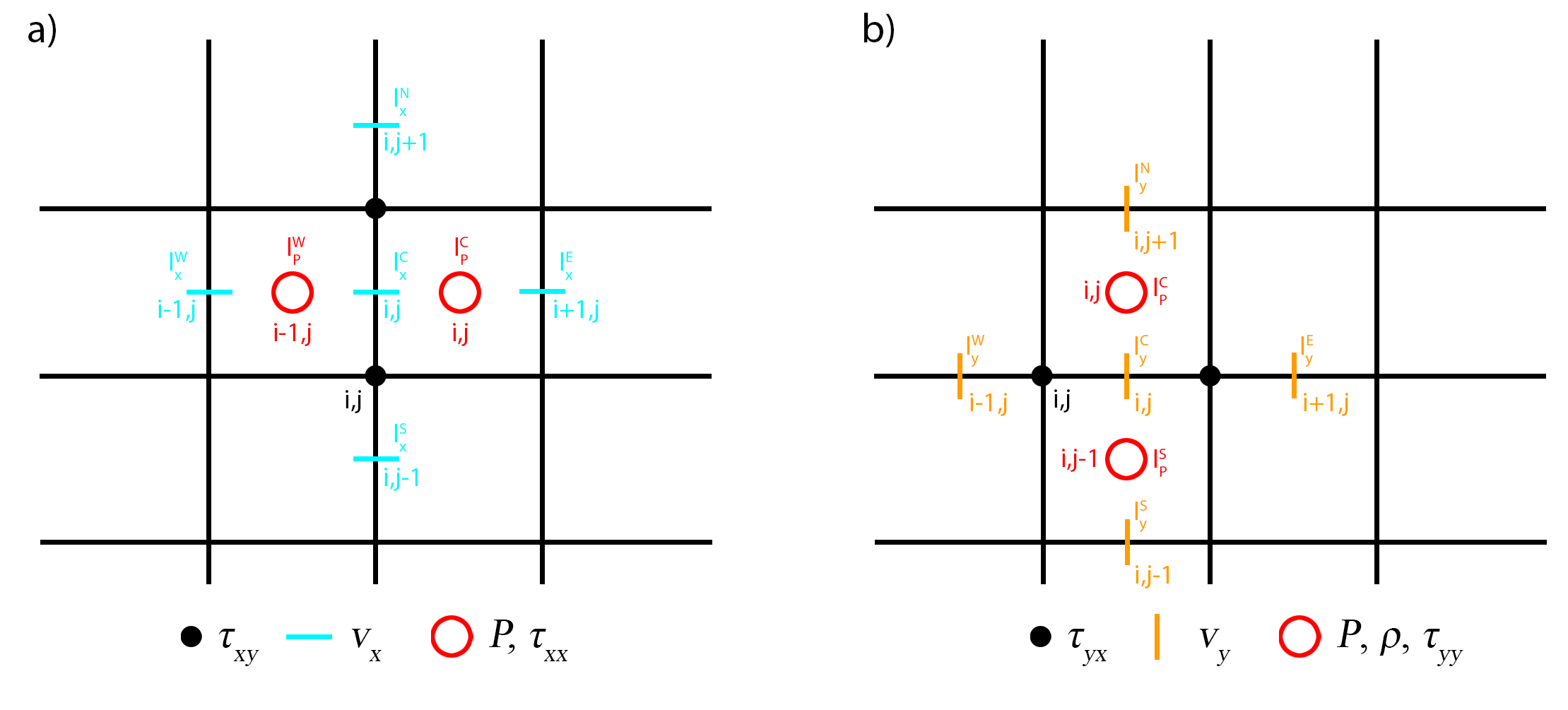
Figure 2. Numerical stencils for constant viscosity. a) $x$-component; b) $y$-component.

By applying finite difference approximations to the partial derivatives, Equations (39) and (40) become:

$x$-component

\[\begin{equation}\begin{gather*} & -\frac{P_{I^{\textrm{C}}_p}-P_{I^{\textrm{W}}_p}}{\Delta{x}} + \\ & \eta\frac{v_{x,I^{\textrm{W}}_{x}}-2v_{x,I^{\textrm{C}}_{x}}+v_{x,I^{\textrm{E}}_{x}}}{\Delta{x^2}} + \\ & \eta\frac{v_{x,I^{\textrm{S}}_{x}}-2v_{x,I^{\textrm{C}}_{x}}+v_{x,I^{\textrm{N}}_{x}}}{\Delta{y^2}} = 0. \end{gather*}\end{equation}\]

Rearranging and grouping terms, we obtain:

\[\begin{equation}\begin{gather*} & W_PP_{I^{\textrm{W}}_{p}} + C_PP_{I^{\textrm{C}}_{p}} + \\ & S_xv_{x,I^{\textrm{S}}_{x}} + W_xv_{x,I^{\textrm{W}}_{x}} + \\ & C_xv_{x,I^{\textrm{C}}_{x}} + \\ & E_xv_{x,I^{\textrm{E}}_{x}} + N_xv_{x,I^{\textrm{N}}_{x}} = 0, \end{gather*}\end{equation}\]

where the coefficients are defined as:

\[\begin{equation} \begin{split} W_P & = \frac{1}{\Delta{x}}, \\ C_P & = -\frac{1}{\Delta{x}}, \\ S_x & = \frac{\eta}{\Delta{y^2}}, \\ W_x & = \frac{\eta}{\Delta{x^2}}, \\ C_x & = -2\eta\left(\frac{1}{\Delta{x^2}}+\frac{1}{\Delta{y^2}}\right), \\ E_x & = \frac{\eta}{\Delta{x^2}}, \\ N_x & = \frac{\eta}{\Delta{y^2}}. \\ \end{split} \end{equation}\]

$y$-component

\[\begin{equation}\begin{gather*} & -\frac{P_{I^{\textrm{C}}_{p}}-P_{I^{\textrm{S}}_{p}}}{\Delta{y}} + \\ & \eta\frac{v_{y,I^{\textrm{S}}_{y}}-2v_{y,I^{\textrm{C}}_{y}}+v_{y,I^{\textrm{N}}_{y}}}{\Delta{y^2}} + \\ & \eta\frac{v_{y,I^{\textrm{W}}_{y}}-2v_{y,I^{\textrm{C}}_{y}}+v_{y,I^{\textrm{E}}_{y}}}{\Delta{x^2}} = \\ & -\frac{\rho_{I^{\textrm{C}}_c}+\rho_{I^{\textrm{S}}_c}}{2} g_y. \end{gather*}\end{equation}\]

Rearranging and grouping terms, we obtain:

\[\begin{equation}\begin{gather*} & S_PP_{I^{\textrm{S}}_{p}} + C_PP_{I^{\textrm{C}}_{p}} + \\ & S_yv_{y,I^{\textrm{S}}_{y}} + W_yv_{y,I^{\textrm{W}}_{y}} + \\ & C_yv_{y,I^{\textrm{C}}_{y}} + \\ & E_yv_{y,I^{\textrm{E}}_{y}} + N_y v_{y,I^{\textrm{N}}_{y}} = \\ & -\frac{\rho_{I^{\textrm{C}}_c}+\rho_{I^{\textrm{S}}_c}}{2} g_y, \end{gather*}\end{equation}\]

with coefficients defined as:

\[\begin{equation} \begin{split} S_P & = \frac{1}{\Delta{y}}, \\ C_P & = -\frac{1}{\Delta{y}}, \\ S_y & = \frac{\eta}{\Delta{y^2}}, \\ W_y & = \frac{\eta}{\Delta{x^2}}, \\ C_y & = -2\eta\left(\frac{1}{\Delta{x^2}}+\frac{1}{\Delta{y^2}}\right), \\ E_y & = \frac{\eta}{\Delta{x^2}}, \\ N_y & = \frac{\eta}{\Delta{y^2}}. \\ \end{split} \end{equation}\]

Variable Viscosity

For variable viscosity, the momentum equation can be written in component form as

$x$-component

\[\begin{equation} -\frac{\partial{P}}{\partial{x}} + \frac{\partial{}}{\partial{x}}\left(2\eta_c\frac{\partial{v_x}}{\partial{x}}\right)+\frac{\partial{}}{\partial{y}}\left( \eta_v\left(\frac{\partial{v_x}}{\partial{y}} + \frac{\partial{v_y}}{\partial{x}}\right)\right) = 0, \end{equation}\]

$y$-component

\[\begin{equation} -\frac{\partial{P}}{\partial{y}} + \frac{\partial{}}{\partial{y}}\left(2\eta_c\frac{\partial{v_y}}{\partial{y}}\right)+\frac{\partial{}}{\partial{x}}\left( \eta_v\left(\frac{\partial{v_y}}{\partial{x}} + \frac{\partial{v_x}}{\partial{y}}\right)\right) = -\frac{\rho_{I^{\textrm{C}}_c}+\rho_{I^{\textrm{S}}_c}}{2}g_y, \end{equation}\]

where $\eta_c$ denotes the viscosity defined at the centroids, and $\eta_v$ denotes the viscosity defined at the vertices.

Stencil

The stencils for the variable-viscosity momentum equations illustrate the grid points required to discretize each velocity component using finite differences (Figure 3).

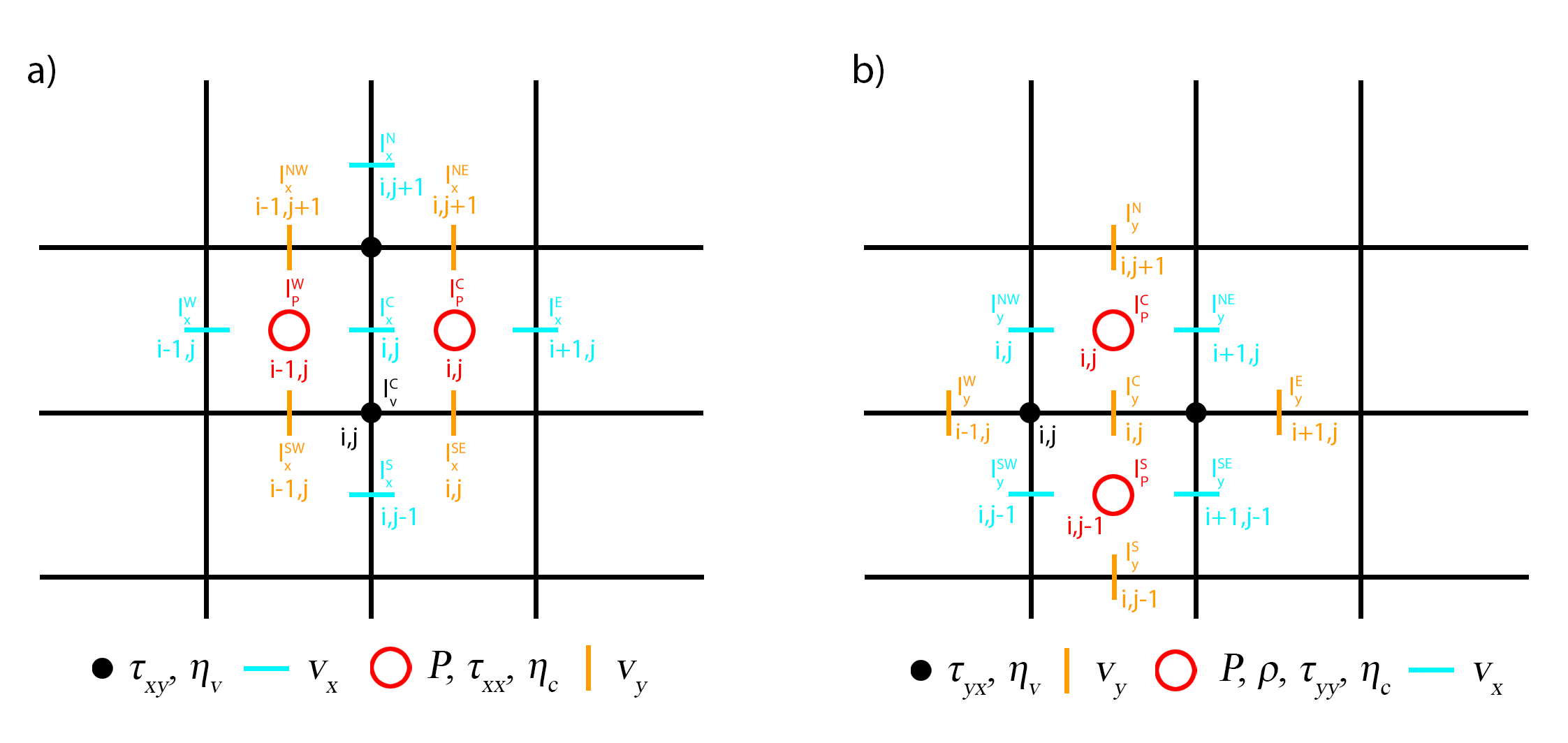
Figure 3. Numerical stencils for variable viscosity. a) $x$-component; b) $y$-component.

Using finite difference approximations, the momentum equations become:

$x$-component

\[\begin{equation} -\frac{P_{I^\textrm{C}_p}-P_{I^\textrm{W}_p}}{\Delta{x}}+\frac{\tau_{xx,I^\textrm{C}_c} -\tau_{xx,I^\textrm{W}_c}}{\Delta{x}} + \frac{\tau_{xy,I^\textrm{N}_v}-\tau_{xy,I^\textrm{C}_v}}{\Delta{y}} = 0, \end{equation}\]

or, explicitly in terms of partial derivatives:

\[\begin{equation}\begin{gather*} & -\frac{P_{I^\textrm{C}_p}-P_{I^\textrm{W}_p}}{\Delta{x}}+\\ & \frac{2\eta_{c,I^\textrm{C}_c}\frac{\partial{v_x}}{\partial{x}}\vert_{I^\textrm{C}_c} -2\eta_{c,I^\textrm{W}_c}\frac{\partial{v_x}}{\partial{x}}\vert_{I^\textrm{W}_c}}{\Delta{x}} + \\ & \frac{\eta_{v,I^\textrm{N}_v}\left(\frac{\partial{v_x}}{\partial{y}}\vert_{I^\textrm{N}_v}+\frac{\partial{v_y}}{\partial{x}}\vert_{I^\textrm{N}_v}\right)-\eta_{v,I^\textrm{C}_v}\left(\frac{\partial{v_x}}{\partial{y}}\vert_{I^\textrm{C}_v}+\frac{\partial{v_y}}{\partial{x}}\vert_{I^\textrm{C}_v}\right)}{\Delta{y}} = 0, \end{gather*}\end{equation}\]

and in terms of the discrete velocity unknowns:

\[\begin{equation}\begin{gather*} & -\frac{P_{I^\textrm{C}_p}-P_{I^\textrm{W}_p}}{\Delta{x}}+ \\ & \frac{2\eta_{c,I^\textrm{C}_c}}{\Delta{x}}\left(\frac{v_{x,I^\textrm{E}_x}-v_{x,I^\textrm{C}_x}}{\Delta{x}}\right) - \\ & \frac{2\eta_{c,I^\textrm{W}_c}}{\Delta{x}}\left(\frac{v_{x,I^\textrm{C}_x}-v_{x,I^\textrm{W}_x}}{\Delta{x}}\right)+ \\ & \frac{\eta_{v,I^\textrm{N}_v}}{\Delta{y}}\left(\frac{v_{x,I^\textrm{N}_x}-v_{x,I^\textrm{C}_x}}{\Delta{y}} + \frac{v_{y,I^\textrm{NE}_x}-v_{y,I^\textrm{NW}_x}}{\Delta{x}}\right) - \\ & \frac{\eta_{v,I^\textrm{C}_v}}{\Delta{y}}\left(\frac{v_{x,I^\textrm{C}_x}-v_{x,I^\textrm{S}_x}}{\Delta{y}} + \frac{v_{y,I^\textrm{SE}_x}-v_{y,I^\textrm{SW}_x}}{\Delta{x}}\right) = 0. \end{gather*}\end{equation}\]

Rearranging and grouping terms yields:

\[\begin{equation}\begin{gather*} & W_PP_{I^\textrm{W}_p}+C_PP_{I^\textrm{C}_p} + \\ & S_xv_{x,I^\textrm{S}_x}+SW_xv_{y,I^\textrm{SW}_x}+SE_xv_{y,I^\textrm{SE}_x}+W_xv_{x,I^\textrm{W}_x}+ \\ & C_xv_{x,I^\textrm{C}_x} + \\ & E_xv_{x,I^\textrm{E}_x} + NW_xv_{y,I^\textrm{NW}_x} + NE_xv_{y,I^\textrm{NE}_x} + N_xv_{x,I^\textrm{N}_x} = \\ & 0, \end{gather*}\end{equation}\]

with coefficients defined as:

\[\begin{equation}\begin{split} W_P & = \frac{1}{\Delta{x}} ,\\ C_P & = -\frac{1}{\Delta{x}}, \\ S_x & = \frac{\eta_{v,I^\textrm{C}_v}}{\Delta{y^2}},\\ SW_x & = \frac{\eta_{v,I^\textrm{C}_v}}{\Delta{x}\Delta{y}},\\ SE_x & = -\frac{\eta_{v,I^\textrm{C}_v}}{\Delta{x}\Delta{y}},\\ W_x & = \frac{2\eta_{c,I^\textrm{W}_c}}{\Delta{x^2}},\\ C_x & = -\frac{2}{\Delta{x^2}}\left(\eta_{c,I^\textrm{C}_c}+\eta_{c,I^\textrm{W}_c}\right)-\frac{1}{\Delta{y^2}}\left(\eta_{v,I^\textrm{N}_v} + \eta_{v,I^\textrm{C}_v} \right), \\ E_x & = \frac{2\eta_{c,I^\textrm{C}_c}}{\Delta{x^2}},\\ NW_x & = -\frac{\eta_{v,I^\textrm{N}_v}}{\Delta{x}\Delta{y}},\\ NE_x & = \frac{\eta_{v,I^\textrm{N}_v}}{\Delta{x}\Delta{y}},\\ N_x & = \frac{\eta_{v,I^\textrm{N}_v}}{\Delta{y^2}}.\\ \end{split}\end{equation}\]

$y$-component

\[\begin{equation} -\frac{P_{I^\textrm{C}_p}-P_{I^\textrm{S}_p}}{\Delta{y}}+\frac{\tau_{yy,I^\textrm{C}_c} - \tau_{yy,I^\textrm{S}_c}}{\Delta{y}} + \frac{\tau_{yx,I^\textrm{E}_v}-\tau_{yx,I^\textrm{C}_v}}{\Delta{x}} = -\frac{\rho_{I^\textrm{C}_c}+\rho_{I^\textrm{S}_c}}{2} g_y, \end{equation}\]

or, expanded:

\[\begin{equation}\begin{gather*} & -\frac{P_{I^\textrm{C}_p}-P_{I^\textrm{S}_p}}{\Delta{y}}+ \\ & \frac{2\eta_{c,I^\textrm{C}_c}\frac{\partial{v_y}}{\partial{y}}\vert_{I^\textrm{C}_c} -2\eta_{c,I^\textrm{S}_c}\frac{\partial{v_y}}{\partial{y}}\vert_{I^\textrm{S}_c}}{\Delta{y}} + \\ & \frac{\eta_{v,I^\textrm{E}_v}\left(\frac{\partial{v_y}}{\partial{x}}\vert_{I^\textrm{E}_v}+\frac{\partial{v_x}}{\partial{y}}\vert_{I^\textrm{E}_v}\right)-\eta_{v,I^\textrm{C}_v}\left(\frac{\partial{v_y}}{\partial{x}}\vert_{I^\textrm{C}_v}+\frac{\partial{v_x}}{\partial{y}}\vert_{I^\textrm{C}_v}\right)}{\Delta{x}} = \\ & -\frac{\rho_{I^\textrm{C}_c}+\rho_{I^\textrm{S}_c}}{2} g_y, \end{gather*}\end{equation}\]

which becomes in discrete form:

\[\begin{equation}\begin{gather*} & -\frac{P_{I^\textrm{C}_p}-P_{I^\textrm{S}_p}}{\Delta{y}}+ \\ & \frac{2\eta_{c,I^\textrm{C}_c}}{\Delta{y}}\left(\frac{v_{y,I^\textrm{N}_y}-v_{y,I^\textrm{C}_y}}{\Delta{y}}\right) - \\ & \frac{2\eta_{c,I^\textrm{S}_c}}{\Delta{y}}\left(\frac{v_{y,I^\textrm{C}_y}-v_{y,I^\textrm{S}_y}}{\Delta{y}}\right)+ \\ & \frac{\eta_{v,I^\textrm{E}_v}}{\Delta{x}}\left(\frac{v_{y,I^\textrm{E}_y}-v_{y,I^\textrm{C}_y}}{\Delta{x}} + \frac{v_{x,I^\textrm{NE}_y}-v_{x,I^\textrm{SE}_y}}{\Delta{y}}\right) - \\ & \frac{\eta_{v,I^\textrm{C}_v}}{\Delta{x}}\left(\frac{v_{y,I^\textrm{C}_y}-v_{y,I^\textrm{W}_y}}{\Delta{x}} + \frac{v_{x,I^\textrm{NW}_y}-v_{x,I^\textrm{SW}_y}}{\Delta{y}}\right) = \\ & -\frac{\rho_{I^\textrm{C}_c}+\rho_{I^\textrm{S}_c}}{2} g_y. \end{gather*}\end{equation}\]

Reorganized:

\[\begin{equation}\begin{gather*} & S_PP_{I^\textrm{S}_p} +C_PP_{I^\textrm{C}_p}+ \\ & S_yv_{y,I^\textrm{S}_y}+SW_yv_{x,I^\textrm{SW}_y}+SE_yv_{x,I^\textrm{SE}_y}+W_yv_{y,I^\textrm{W}_y}+ \\ & C_yv_{y,I^\textrm{C}_y} + \\ & E_yv_{y,I^\textrm{E}_y} + NW_yv_{x,I^\textrm{NW}_y} + NE_yv_{x,I^\textrm{NE}_y} + N_yv_{y,I^\textrm{N}_y} = \\ & -\frac{\rho_{I^\textrm{C}_c}+\rho_{I^\textrm{S}_c}}{2} g_y, \end{gather*}\end{equation}\]

with coefficients:

\[\begin{equation}\begin{split} S_P & = \frac{1}{\Delta{y}}, \\ C_P & = -\frac{1}{\Delta{y}}, \\ S_y & = \frac{2\eta_{c,I^\textrm{S}_c}}{\Delta{y^2}},\\ SW_y & = \frac{\eta_{v,I^\textrm{C}_v}}{\Delta{x}\Delta{y}},\\ SE_y & = -\frac{\eta_{v,I^\textrm{E}_v}}{\Delta{x}\Delta{y}},\\ W_y & = \frac{\eta_{v,I^\textrm{C}_v}}{\Delta{x^2}},\\ C_y & = -\frac{2}{\Delta{y^2}}\left(\eta_{c,I^\textrm{C}_c}+\eta_{c,I^\textrm{S}_c}\right)-\frac{1}{\Delta{x^2}}\left(\eta_{v,I^\textrm{E}_v} + \eta_{v,I^\textrm{C}_v} \right), \\ E_y & = \frac{\eta_{v,I^\textrm{E}_v}}{\Delta{x^2}},\\ NW_y & = -\frac{\eta_{v,I^\textrm{C}_v}}{\Delta{x}\Delta{y}},\\ NE_y & = \frac{\eta_{v,I^\textrm{E}_v}}{\Delta{x}\Delta{y}},\\ N_y & = \frac{2\eta_{c,I^\textrm{C}_c}}{\Delta{y^2}}.\\ \end{split}\end{equation}\]

For more details on the implementation, please refer to the source code.

Continuity Equation

The mass conservation equation provides the additional constraint required to solve for the pressure field.

Stencil

The corresponding numerical stencil involves only the horizontal and vertical velocity components (Figure 4).

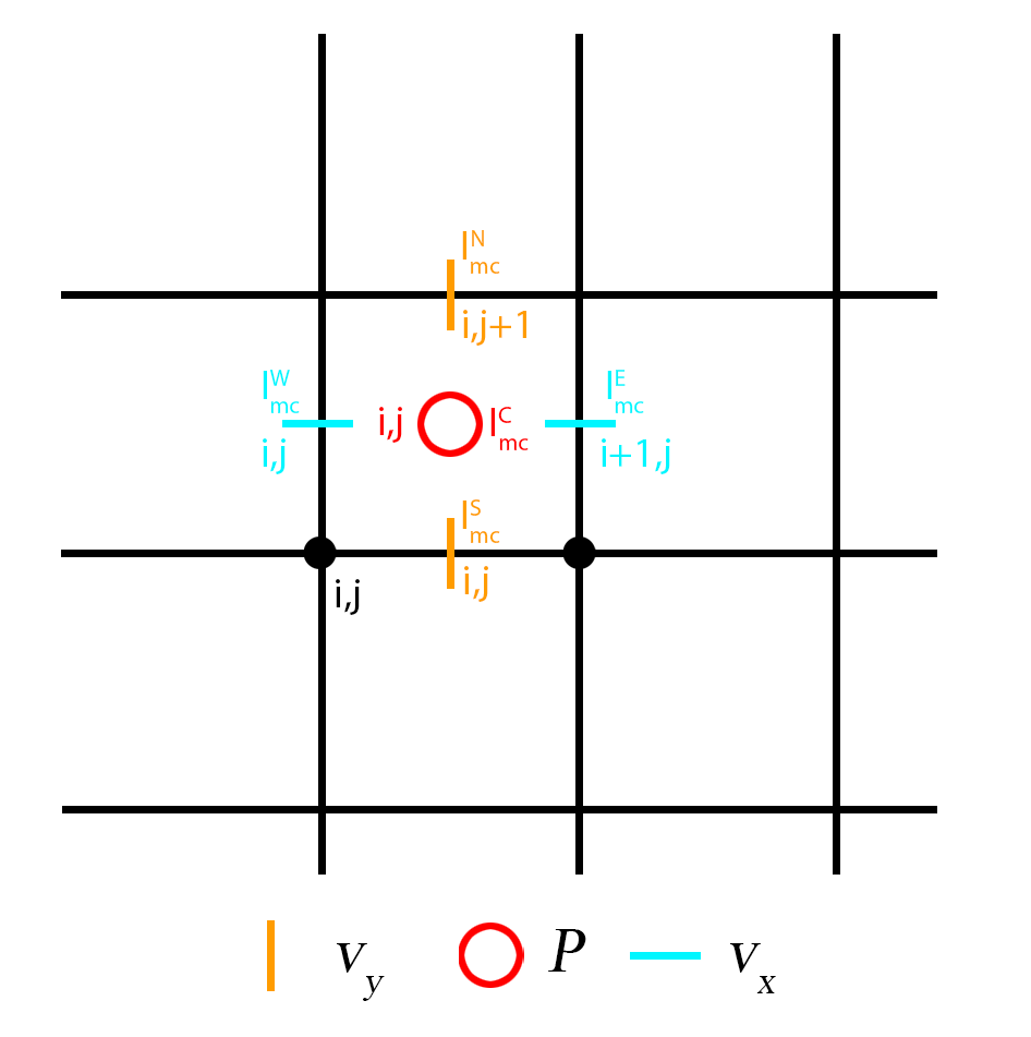
Figure 4. Numerical stencil for the continuity equation.

Using the finite difference operators, equation (6) is defined as:

\[\begin{equation} \frac{v_{x,I^\textrm{E}_{mc}}-v_{x,I^\textrm{W}_{mc}}}{\Delta{x}} + \frac{v_{y,I^\textrm{N}_{mc}}-v_{y,I^\textrm{S}_{mc}}}{\Delta{y}} = 0, \end{equation}\]

\[\begin{equation} W_{mc}v_{x,I^\textrm{W}_{mc}} + E_{mc}v_{x,I^\textrm{E}_{mc}} + S_{mc}v_{y,I^\textrm{S}_{mc}} + N_{mc}v_{y,I^\textrm{N}_{mc}} = 0, \end{equation}\]

with

\[\begin{equation} \begin{split} W_{mc} = -\frac{1}{\Delta{x}}, \qquad E_{mc} = \frac{1}{\Delta{x}}, \\ S_{mc} = -\frac{1}{\Delta{y}}, \qquad N_{mc} = \frac{1}{\Delta{y}}. \end{split} \end{equation}\]

Solution

Following the discretization described above, the equations form a linear system with 7 non-zero diagonals for constant viscosity and 11 non-zero diagonals for variable viscosity:

\[\begin{equation} \mathbf{K} \cdot \mathbf{x} = \mathbf{b}, \end{equation}\]

where $\mathbf{K}$ is the coefficient matrix, $\mathbf{x}$ is the solution vector, and $\mathbf{b}$ is the known right-hand side.

The solution vector contains the horizontal and vertical velocity as well as the pressure field, whose ordering follows the system global numbering of $I^\textrm{C}_x$, $I^\textrm{C}_y$, and $I^\textrm{C}_p$ as defined in Equations (9)-(11). The right-hand side contains the buoyancy term for the $y$-component of the momentum equation. Depending on the chosen solution strategy, it may also include contributions from the boundary conditions.

The coefficient matrix $\mathbf{K_{I^\textrm{C}_{i},I^k_{j}}}$ varies depending on the state of the viscosity. The structure of the coefficient matrix for a certain grid resolution and boundary condition is shown in Figures (5) and (6).

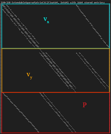
Figure 5. Coefficient matrix, constant viscosity. Non-zero entries of a coefficient matrix for a resolution of $nc_x=nc_y=10$, a constant viscosity, and free-slip boundaries. Highlighted are the areas for the different equations: $v_x$ - $x$-component of the momentum equation, $v_y$ - $y$-component of the momentum equation, $P$ - continuity equation.

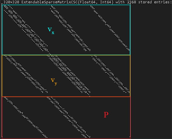
Figure 6. Coefficient matrix, variable viscosity. Non-zero entries of a coefficient matrix for a resolution of $nc_x=nc_y=10$, a variable viscosity, and free-slip boundaries. Highlighted are the areas for the different equations: $v_x$ - $x$-component of the momentum equation, $v_y$ - $y$-component of the momentum equation, $P$ - continuity equation.

General Solution - Defect Correction

The system of equations can be solved in a general way using the defect correction. The equations are reformulated by introducing a residual term $\mathbf{r}$, which quantifies the deviation from the true solution and can be reduced iteratively to improve accuracy through successive correction steps. The defect correction method is particularly effective when solving non-linear systems.

First, the residual is calculated for each equation. If the velocity nodes required to calculate the residual are not located directly on the boundary, the corresponding ghost-node velocity values defined in Equations (21)-(37) are used. The stresses are either calculated via the shear (vertices) or the normal viscosity (centroids).

The residuals $r_x$, $r_y$, and $r_p$ denote the local residuals at the corresponding central reference nodes of each variable grid. To solve the system of equations, the residuals are stored in a vector $\mathbf{r}$ with the global indexing as shown in Equations (9)-(11).

The local residual at the central reference node is defined as:

Residual calculation

\[\begin{equation}\begin{split} r_x & = \frac{\partial{\tau_{xx}}}{\partial{x}} + \frac{\partial{\tau_{xy}}}{\partial{y}} - \frac{\partial{P}}{\partial{x}}, \\ r_y & = \frac{\partial{\tau_{yy}}}{\partial{y}} + \frac{\partial{\tau_{yx}}}{\partial{x}} - \frac{\partial{P}}{\partial{y}} + \rho g_y, \\ r_p & = \frac{\partial{v_x}}{\partial{x}} + \frac{\partial{v_y}}{\partial{y}}, \end{split}\end{equation}\]

and in the form the finite difference operators:

\[\begin{equation}\begin{split} r_{I^\textrm{C}_x} & = \frac{\tau_{xx,I^\textrm{C}_c}-\tau_{xx,I^\textrm{W}_c}}{\Delta{x}} + \frac{\tau_{xy,I^\textrm{N}_v}-\tau_{xy,I^\textrm{C}_v}}{\Delta{y}} - \frac{P_{I^\textrm{C}_p}-P_{I^\textrm{W}_p}}{\Delta{x}}, \\ r_{I^\textrm{C}_y} & = \frac{\tau_{yy,I^\textrm{C}_c}-\tau_{yy,I^\textrm{S}_c}}{\Delta{y}} + \frac{\tau_{yx,I^\textrm{E}_v}-\tau_{yx,I^\textrm{C}_v}}{\Delta{x}} - \frac{P_{I^\textrm{C}_p}-P_{I^\textrm{S}_p}}{\Delta{y}} + \frac{\rho_{I^\textrm{C}_c}+\rho_{I^\textrm{S}_c}}{2} g_y, \\ r_{I^\textrm{C}_p} & = \frac{v_{x,I^\textrm{E}_{mc}}-v_{x,I^\textrm{W}_{mc}}}{\Delta{x}} + \frac{v_{y,I^\textrm{N}_{mc}}-v_{y,I^\textrm{S}_{mc}}}{\Delta{y}}. \end{split}\end{equation}\]

Or in the terms of the unknown variables:

Constant Viscosity

$x$-component

\[\begin{equation}\begin{gather*} & r_{I^\textrm{C}_x} = W_PP_{I^{\textrm{W}}_{p}} + C_PP_{I^{\textrm{C}}_{p}} + \\ & S_xv_{x,I^{\textrm{S}}_{x}} + W_xv_{x,I^{\textrm{W}}_{x}} + C_xv_{x,I^{\textrm{C}}_{x}} + E_xv_{x,I^{\textrm{E}}_{x}} + N_xv_{x,I^{\textrm{N}}_{x}}, \end{gather*}\end{equation}\]

$y$-component

\[\begin{equation}\begin{gather*} & r_{I^\textrm{C}_y} = S_PP_{I^{\textrm{S}}_{p}} + C_PP_{I^{\textrm{C}}_{p}} + \\ & S_yv_{y,I^{\textrm{S}}_{y}} + W_yv_{y,I^{\textrm{W}}_{y}} + C_yv_{y,I^{\textrm{C}}_{y}} + E_yv_{y,I^{\textrm{E}}_{y}} + N_y v_{y,I^{\textrm{N}}_{y}} +\frac{\rho_{I^{\textrm{C}}_c}+\rho_{I^{\textrm{S}}_c}}{2} g_y, \end{gather*}\end{equation}\]

Variable Viscosity

$x$-component

\[\begin{equation}\begin{gather*} & r_{I^\textrm{C}_x} = W_PP_{I^\textrm{W}_p}+C_PP_{I^\textrm{C}_p} + \\ & S_xv_{x,I^\textrm{S}_x}+SW_xv_{y,I^\textrm{SW}_x}+SE_xv_{y,I^\textrm{SE}_x}+W_xv_{x,I^\textrm{W}_x}+ \\ & C_xv_{x,I^\textrm{C}_x} + E_xv_{x,I^\textrm{E}_x} + NW_xv_{y,I^\textrm{NW}_x} + NE_xv_{y,I^\textrm{NE}_x} + N_xv_{x,I^\textrm{N}_x}, \end{gather*}\end{equation}\]

$y$-component

\[\begin{equation}\begin{gather*} & r_{I^\textrm{C}_y} = S_PP_{I^\textrm{S}_p} +C_PP_{I^\textrm{C}_p}+ \\ & S_yv_{y,I^\textrm{S}_y}+SW_yv_{x,I^\textrm{SW}_y}+SE_yv_{x,I^\textrm{SE}_y}+W_yv_{y,I^\textrm{W}_y}+ \\ & C_yv_{y,I^\textrm{C}_y} + E_yv_{y,I^\textrm{E}_y} + NW_yv_{x,I^\textrm{NW}_y} + NE_yv_{x,I^\textrm{NE}_y} + N_yv_{y,I^\textrm{N}_y} + \frac{\rho_{I^\textrm{C}_c}+\rho_{I^\textrm{S}_c}}{2} g_y, \end{gather*}\end{equation}\]

Continuity Equation

\[\begin{equation} r_{I^\textrm{C}_p} = W_{mc}v_{x,I^\textrm{W}_{mc}} + E_{mc}v_{x,I^\textrm{E}_{mc}} + S_{mc}v_{y,I^\textrm{S}_{mc}} + N_{mc}v_{y,I^\textrm{N}_{mc}}. \end{equation}\]

For more details on the defect correction method for the Stokes equation see the 1-D Stokes equation documentation.

The correction vector $\delta$ for the velocity components and the pressure, is obtained by solving the linear system:

\[\begin{equation} \mathbf{\delta}=- \mathbf{K}^{-1} \mathbf{r}. \end{equation}\]

The vector $\delta$ has a length equal to the total number of unknowns, i.e., $\left(nv_x \cdot nc_y + nc_x \cdot nv_y + nc_x \cdot nc_y\right)$, corresponding to $v_x$, $v_y$, and $P$ across the domain.

Finally one needs to update the initial guess by the correction term:

\[\begin{equation}\begin{split} v_{x,I^\textrm{C}_x}^{k+1} & = v_{x,I^\textrm{C}_x}^k + \delta_{I^\textrm{C}_x}, \\ v_{y,I^\textrm{C}_y}^{k+1} & = v_{y,I^\textrm{C}_y}^k + \delta_{I^\textrm{C}_y}, \\ P_{I^\textrm{C}_p}^{k+1} & = P_{I^\textrm{C}_p}^k + \delta_{I^\textrm{C}_p}, \end{split}\end{equation}\]

where the index of the vector $\delta$ corresponds to the global index for the variables as shown in Equations (9)-(11).

Boundary Conditions

The boundary conditions are implemented using the velocity values at the ghost nodes (see Equations (21)-(31)). Substituting the ghost-node values into the discretized equations modifies the coefficients of the equations adjacent to the domain boundaries while preserving the stencil structure. For simplicity, we focus here on the two most common boundary conditions, no-slip and free-slip. The constant-velocity and pure-shear boundary conditions are implemented using the same ghost-node substitutions as the no-slip and free-slip conditions, respectively, and therefore lead to analogous modifications of the discretized equations. The resulting equations for the control volumes adjacent to the boundaries are given by:

Constant Viscosity

Free-slip

Using Equations (21)-(26), the discretized system of equations is updated accordingly. For free-slip boundaries, the right-hand side remains unchanged, but the coefficients are modified.

$x$-component

South

\[\begin{equation}\begin{gather*} & r_{I^\textrm{C}_x} = W_PP_{I^{\textrm{W}}_{p}}+C_PP_{I^{\textrm{C}}_{p}}+ \\ & W_xv_{x,I^{\textrm{W}}_{x}} + C_xv_{x,I^{\textrm{C}}_{x}}+ E_xv_{x,I^{\textrm{E}}_{x}}+N_xv_{x,I^{\textrm{N}}_{x}}, \end{gather*}\end{equation}\]

with

\[\begin{equation}C_x = -\frac{2\eta}{\Delta{x^2}}-\frac{\eta}{\Delta{y^2}}.\end{equation}\]

North

\[\begin{equation}\begin{gather*} & r_{I^\textrm{C}_x} = W_PP_{I^{\textrm{W}}_{p}}+C_PP_{I^{\textrm{C}}_{p}}+ \\ & S_xv_{x,I^{\textrm{S}}_{x}}+ W_xv_{x,I^{\textrm{W}}_{x}}+ C_xv_{x,I^{\textrm{C}}_{x}} + E_xv_{x,I^{\textrm{E}}_{x}} , \end{gather*}\end{equation}\]

with

\[\begin{equation}C_x = -\frac{2\eta}{\Delta{x^2}}-\frac{\eta}{\Delta{y^2}}.\end{equation}\]

On the lateral boundaries (East, West), the central coefficient is set to:

\[\begin{equation} C_x = 1, \end{equation}\]

and all other coefficients are set to zero.

$y$-component

West

\[\begin{equation}\begin{gather*} & r_{I^\textrm{C}_y} = S_PP_{I^{\textrm{S}}_{p}}+C_PP_{I^{\textrm{C}}_{p}}+ \\ & S_yv_{y,I^{\textrm{S}}_{y}} + C_yv_{y,I^{\textrm{C}}_{y}}+ E_yv_{y,I^{\textrm{E}}_{y}}+ N_yv_{y,I^{\textrm{N}}_{y}} + \frac{\rho_{I^{\textrm{C}}_c}+\rho_{I^{\textrm{S}}_c}}{2} g_y, \end{gather*}\end{equation}\]

with

\[\begin{equation}C_y = -\frac{\eta}{\Delta{x^2}}-\frac{2\eta}{\Delta{y^2}}.\end{equation}\]

East

\[\begin{equation}\begin{gather*} & r_{I^\textrm{C}_y} = S_PP_{I^{\textrm{S}}_{p}}+C_PP_{I^{\textrm{C}}_{p}}+ \\ & S_yv_{y,I^{\textrm{S}}_{y}}+ W_yv_{y,I^{\textrm{W}}_{y}}+ C_yv_{y,I^{\textrm{C}}_{y}} + N_yv_{y,I^{\textrm{N}}_{y}} + \frac{\rho_{I^{\textrm{C}}_c}+\rho_{I^{\textrm{S}}_c}}{2} g_y, \end{gather*}\end{equation}\]

with

\[\begin{equation}C_y = -\frac{\eta}{\Delta{x^2}}-\frac{2\eta}{\Delta{y^2}}.\end{equation}\]

On the North and South boundaries, the central coefficient is:

\[\begin{equation} C_y = 1, \end{equation}\]

and all other coefficients are zero.

No-slip

Using Equations (27)-(31), the system coefficients and the right-hand side of the discretized equations are modified accordingly.

$x$-component

South

\[\begin{equation}\begin{gather*} & r_{I^\textrm{C}_x} = W_PP_{I^{\textrm{W}}_{p}}+C_PP_{I^{\textrm{C}}_{p}}+ \\ & W_xv_{x,I^{\textrm{W}}_{x}} + C_xv_{x,I^{\textrm{C}}_{x}}+ E_xv_{x,I^{\textrm{E}}_{x}}+N_xv_{x,I^{\textrm{N}}_{x}} + 2\frac{\eta}{\Delta{y^2}}V_{BC}^S, \end{gather*}\end{equation}\]

with

\[\begin{equation}C_x = -\frac{2\eta}{\Delta{x^2}}-\frac{3\eta}{\Delta{y^2}}.\end{equation}\]

North

\[\begin{equation}\begin{gather*} & r_{I^\textrm{C}_x} = W_PP_{I^{\textrm{W}}_{p}}+C_PP_{I^{\textrm{C}}_{p}}+ \\ & S_xv_{x,I^{\textrm{S}}_{x}}+W_xv_{x,I^{\textrm{W}}_{x}}+ C_xv_{x,I^{\textrm{C}}_{x}} + E_xv_{x,I^{\textrm{E}}_{x}} + 2\frac{\eta}{\Delta{y^2}}V_{BC}^N, \end{gather*}\end{equation}\]

with

\[\begin{equation}C_x = -\frac{2\eta}{\Delta{x^2}}-\frac{3\eta}{\Delta{y^2}}.\end{equation}\]

On the lateral boundaries (East, West), set:

\[\begin{equation} C_x = 1, \end{equation}\]

with all other coefficients and the right-hand side equal to zero.

$y$-component

West

\[\begin{equation}\begin{gather*} & r_{I^\textrm{C}_y} = S_PP_{I^{\textrm{S}}_{p}}+C_PP_{I^{\textrm{C}}_{p}}+ \\ & S_yv_{y,I^{\textrm{S}}_{y}}+ C_yv_{y,I^{\textrm{C}}_{y}}+ E_yv_{y,I^{\textrm{E}}_{y}}+N_yv_{y,I^{\textrm{N}}_{y}} + \frac{\rho_{I^{\textrm{C}}_c} + \rho_{I^{\textrm{S}}_c}}{2} g_y + 2\frac{\eta}{\Delta{x^2}}V_{BC}^W, \end{gather*}\end{equation}\]

with

\[\begin{equation}C_y = -\frac{3\eta}{\Delta{x^2}}-\frac{2\eta}{\Delta{y^2}}.\end{equation}\]

East

\[\begin{equation}\begin{gather*} & r_{I^\textrm{C}_y} = S_PP_{I^{\textrm{S}}_{p}}+C_PP_{I^{\textrm{C}}_{p}}+ \\ & S_yv_{y,I^{\textrm{S}}_{y}}+W_yv_{y,I^{\textrm{W}}_{y}}+ C_yv_{y,I^{\textrm{C}}_{y}} + N_yv_{y,I^{\textrm{N}}_{y}} + \frac{\rho_{I^{\textrm{C}}_c} + \rho_{I^{\textrm{S}}_c}}{2} g_y + 2\frac{\eta}{\Delta{x^2}}V_{BC}^E, \end{gather*}\end{equation}\]

with

\[\begin{equation}C_y = -\frac{3\eta}{\Delta{x^2}}-\frac{2\eta}{\Delta{y^2}}.\end{equation}\]

On the horizontal boundaries (North, South), set:

\[\begin{equation} C_y = 1, \end{equation}\]

and all other coefficients and the right-hand side to zero.

For implementation details, please refer to the source code.

Variable Viscosity

Free-slip

Using Equations (21)-(26), the coefficients of the equations adjacent to the corresponding boundaries are modified accordingly. Note that the right-hand side does not change for free-slip boundary conditions.

$x$-component

South

\[\begin{equation}\begin{gather*} & r_{I^{\textrm{C}}_x} = W_PP_{I^{\textrm{W}}_p} + C_PP_{I^{\textrm{C}}_p} +\\ & SW_xv_{y,I^{\textrm{SW}}_x}+SE_xv_{y,I^{\textrm{SE}}_x}+W_xv_{x,I^{\textrm{W}}_x}+\\ & C_xv_{x,I^{\textrm{C}}_x}+ E_xv_{x,I^{\textrm{E}}_x}+NW_xv_{y,I^{\textrm{NW}}_x}+NE_xv_{y,I^{\textrm{NE}}_x}+N_xv_{x,I^{\textrm{N}}_x}, \end{gather*}\end{equation}\]

with

\[\begin{equation}C_x = -\frac{2}{\Delta{x^2}} \left( \eta_{c,I^{\textrm{C}}_c} + \eta_{c,I^{\textrm{W}}_c} \right) - \frac{\eta_{v,I^{\textrm{N}}_v}}{\Delta{y^2}}.\end{equation}\]

North

\[\begin{equation}\begin{gather*} & r_{I^{\textrm{C}}_x} = W_PP_{I^{\textrm{W}}_p}+C_PP_{I^{\textrm{C}}_p}+\\ & S_xv_{x,I^{\textrm{S}}_x}+SW_xv_{y,I^{\textrm{SW}}_x}+SE_xv_{y,I^{\textrm{SE}}_x}+W_xv_{x,I^{\textrm{W}}_x}+ \\ & C_xv_{x,I^{\textrm{C}}_x}+ E_xv_{x,I^{\textrm{E}}_x}+NW_xv_{y,I^{\textrm{NW}}_x}+NE_xv_{y,I^{\textrm{NE}}_x}, \end{gather*}\end{equation}\]

with

\[\begin{equation}C_x = -\frac{2}{\Delta{x^2}}\left(\eta_{c,I^{\textrm{C}}_c}+\eta_{c,I^{\textrm{W}}_c}\right)-\frac{\eta_{v,I^{\textrm{C}}_v}}{\Delta{y^2}}.\end{equation}\]

Along the lateral boundaries (East, West), the central coefficient is set to:

\[\begin{equation} C_x = 1, \end{equation}\]

and all other coefficients are set to zero.

$y$-component

West

\[\begin{equation}\begin{gather*} & r_{I^{\textrm{C}}_y} = C_PP_{I^{\textrm{C}}_p}+S_PP_{I^{\textrm{S}}_p} + \\ & S_yv_{y,I^{\textrm{S}}_y} + SW_yv_{x,I^{\textrm{SW}}_y} + SE_yv_{x,I^{\textrm{SE}}_y} + \\ & C_yv_{y,I^{\textrm{C}}_y} + E_yv_{y,I^{\textrm{E}}_y} + NW_yv_{x,I^{\textrm{NW}}_y} + NE_yv_{x,I^{\textrm{NE}}_y} + N_yv_{y,I^{\textrm{N}}_y} + \frac{\rho_{I^{\textrm{C}}_c}+\rho_{I^{\textrm{S}}_c}}{2} g_y, \end{gather*}\end{equation}\]

with

\[\begin{equation}C_y = -\frac{2}{\Delta{y^2}}\left(\eta_{c,I^{\textrm{C}}_c}+\eta_{c,I^{\textrm{S}}_c}\right)-\frac{\eta_{v,I^{\textrm{E}}_v}}{\Delta{x^2}}.\end{equation}\]

East

\[\begin{equation}\begin{gather*} & r_{I^{\textrm{C}}_y} = C_PP_{I^{\textrm{C}}_p} + S_PP_{I^{\textrm{S}}_p} + \\ & S_yv_{y,I^{\textrm{S}}_y} + SW_yv_{x,I^{\textrm{SW}}_y} + SE_yv_{x,I^{\textrm{SE}}_y} + W_yv_{y,I^{\textrm{W}}_y} + \\ & C_yv_{y,I^{\textrm{C}}_y} + NW_yv_{x,I^{\textrm{NW}}_y} + NE_yv_{x,I^{\textrm{NE}}_y} + N_yv_{y,I^{\textrm{N}}_y} + \frac{\rho_{I^{\textrm{C}}_c}+\rho_{I^{\textrm{S}}_c}}{2} g_y, \end{gather*}\end{equation}\]

with

\[\begin{equation}C_y = -\frac{2}{\Delta{y^2}}\left(\eta_{c,I^{\textrm{C}}_c}+\eta_{c,I^{\textrm{S}}_c}\right)-\frac{\eta_{v,I^{\textrm{C}}_v}}{\Delta{x^2}}.\end{equation}\]

Along the horizontal boundaries (North, South), the central coefficient is set to:

\[\begin{equation} C_y = 1, \end{equation}\]

and all other coefficients are set to zero.

No-slip

Using Equations (27)-(31), the coefficients of the equations adjacent to the corresponding boundaries and the right-hand side change as

$x$-component

South

\[\begin{equation}\begin{gather*} & r_{I^{\textrm{C}}_x} = W_PP_{I^{\textrm{W}}_p}+C_PP_{I^{\textrm{C}}_p}+ \\ & SW_xv_{y,I^{\textrm{SW}}_x}+SE_xv_{y,I^{\textrm{SE}}_x}+W_xv_{x,I^{\textrm{W}}_x}+ \\ & C_xv_{x,I^{\textrm{C}}_x}+ E_xv_{x,I^{\textrm{E}}_x}+NW_xv_{y,I^{\textrm{NW}}_x}+NE_xv_{y,I^{\textrm{NE}}_x}+N_xv_{x,I^{\textrm{N}}_x} + 2\frac{\eta_{v,I^{\textrm{C}}_v}}{\Delta{y^2}}V_{BC}^S, \end{gather*}\end{equation}\]

with

\[\begin{equation}C_x = -\frac{2}{\Delta{x^2}}\left(\eta_{c,I^{\textrm{C}}_c}+\eta_{c,I^{\textrm{W}}_c}\right)-\frac{\eta_{v,I^{\textrm{N}}_v}}{\Delta{y^2}}-\frac{2\eta_{v,I^{\textrm{C}}_v}}{\Delta{y^2}}.\end{equation}\]

North

\[\begin{equation}\begin{gather*} & r_{I^{\textrm{C}}_x} = W_PP_{I^{\textrm{W}}_p}+C_PP_{I^{\textrm{C}}_p}+ \\ & S_xv_{x,I^{\textrm{S}}_x}+SW_xv_{y,I^{\textrm{SW}}_x}+SE_xv_{y,I^{\textrm{SE}}_x}+W_xv_{x,I^{\textrm{W}}_x}+ \\ & C_xv_{x,I^{\textrm{C}}_x}+ E_xv_{x,I^{\textrm{E}}_x}+NW_xv_{y,I^{\textrm{NW}}_x}+NE_xv_{y,I^{\textrm{NE}}_x} + 2\frac{\eta_{v,I^{\textrm{N}}_v}}{\Delta{y^2}}V_{BC}^N, \end{gather*}\end{equation}\]

with

\[\begin{equation}C_x = -\frac{2}{\Delta{x^2}}\left(\eta_{c,I^{\textrm{C}}_c}+\eta_{c,I^{\textrm{W}}_c}\right)-\frac{2\eta_{v,I^{\textrm{N}}_v}}{\Delta{y^2}}-\frac{\eta_{v,I^{\textrm{C}}_v}}{\Delta{y^2}}.\end{equation}\]

Along the lateral boundaries (East, West), the central coefficient is set to:

\[\begin{equation} C_x = 1, \end{equation}\]

and all other coefficients are set to zero.

$y$-component

West

\[\begin{equation}\begin{gather*} & r_{I^{\textrm{C}}_y} = C_PP_{I^{\textrm{C}}_p} + S_PP_{I^{\textrm{S}}_p} + \\ & S_yv_{y,I^{\textrm{S}}_y} + SW_yv_{x,I^{\textrm{SW}}_y} + SE_yv_{x,I^{\textrm{SE}}_y} + \\ & C_yv_{y,I^{\textrm{C}}_y} + E_yv_{y,I^{\textrm{E}}_y} + NW_yv_{x,I^{\textrm{NW}}_y} + NE_yv_{x,I^{\textrm{NE}}_y} + N_yv_{y,I^{\textrm{N}}_y} + \frac{\rho_{I^{\textrm{C}}_c}+\rho_{I^{\textrm{S}}_c}}{2} g_y + 2\frac{\eta_{v,I^{\textrm{C}}_v}}{\Delta{x^2}}V_{BC}^W, \end{gather*}\end{equation}\]

with

\[\begin{equation}C_y = -\frac{2}{\Delta{y^2}}\left(\eta_{c,I^{\textrm{C}}_c}+\eta_{c,I^{\textrm{S}}_c}\right)-\frac{\eta_{v,I^{\textrm{E}}_v}}{\Delta{x^2}}-2\frac{\eta_{v,I^{\textrm{C}}_v}}{\Delta{x^2}}.\end{equation}\]

East

\[\begin{equation}\begin{gather*} & r_{I^{\textrm{C}}_y} = C_PP_{I^{\textrm{C}}_p} + S_PP_{I^{\textrm{S}}_p} + \\ & S_yv_{y,I^{\textrm{S}}_y} + SW_yv_{x,I^{\textrm{SW}}_y} + SE_yv_{x,I^{\textrm{SE}}_y} + W_yv_{y,I^{\textrm{W}}_y} + \\ & C_yv_{y,I^{\textrm{C}}_y} + NW_yv_{x,I^{\textrm{NW}}_y} + NE_yv_{x,I^{\textrm{NE}}_y} + N_yv_{y,I^{\textrm{N}}_y} + \frac{\rho_{I^{\textrm{C}}_c}+\rho_{I^{\textrm{S}}_c}}{2} g_y + 2\frac{\eta_{v,I^{\textrm{E}}_v}}{\Delta{x^2}}V_{BC}^E, \end{gather*}\end{equation}\]

with

\[\begin{equation}C_y = -\frac{2}{\Delta{y^2}}\left(\eta_{c,I^{\textrm{C}}_c}+\eta_{c,I^{\textrm{S}}_c}\right)-\frac{2\eta_{v,I^{\textrm{E}}_v}}{\Delta{x^2}}-\frac{\eta_{v,I^{\textrm{C}}_v}}{\Delta{x^2}}.\end{equation}\]

Along the horizontal boundaries (North, South), the central coefficient is set to:

\[\begin{equation} C_y = 1, \end{equation}\]

and all other coefficients are set to zero.

Although explicitly rewriting the complete equations is mathematically valid, GeoModBox.jl applies the boundary conditions by constructing the appropriate ghost-node velocity values during the residual calculation and by modifying the corresponding coefficients of the assembled matrix. Equations (72)–(111) are provided to illustrate the resulting changes to the matrix coefficients and boundary contributions. These adjustments ensure that the boundary conditions are enforced consistently in both the residual calculation and the assembled linear system.

Special-case Solution

There is also a special case for solving this system of equations when the system is linear. In that case, the system of equations reduces to Equation (62) and can be solved directly via left-matrix division. The coefficient matrices remain the same, even for the given boundary conditions. However, the right-hand side must be updated accordingly by setting $\mathbf{r}=0$ and adding the known terms to the right-hand side of the equations.

For more information on how both methods are implemented see the examples.