Internally Heated Convection
This example demonstrates two-dimensional thermal convection driven by internal radiogenic heating using the finite-difference solvers provided by GeoModBox.jl. In contrast to the bottom-heated convection example, thermal energy is generated uniformly throughout the domain, producing buoyancy forces that drive mantle convection.
The example builds directly upon the bottom-heated convection model and demonstrates how different physical source terms can be incorporated into the same numerical framework. The coupled Stokes and heat equations are solved using adaptive time stepping, semi-Lagrangian advection, and a Crank-Nicolson discretization of the heat equation solved with the general defect-correction framework. Throughout the simulation, diagnostic quantities such as the Nusselt number, the root-mean-square velocity, and the horizontally averaged temperature profile are monitored to characterize the evolution of the convective system.
This example considers internally heated convection with an internal-heating Rayleigh number of
\[\begin{equation} Ra_Q \approx 1.5 \cdot 10^7. \end{equation}\]
The example uses the momentum, advection, and heat-equation solvers of GeoModBox.jl together with standard Julia packages for sparse linear algebra, visualization, and performance measurements.
using Plots, ExtendableSparse
using GeoModBox
using GeoModBox.InitialCondition, GeoModBox.MomentumEquation.TwoD
using GeoModBox.AdvectionEquation.TwoD, GeoModBox.HeatEquation.TwoD
using GeoModBox.Scaling
using Statistics, LinearAlgebra
using Printf, TimerOutputs, LaTeXStrings, Measures
The following section specifies the initial temperature distribution together with several visualization parameters used to generate animations and diagnostic figures during the simulation.
to      =   TimerOutput()
# Define Initial Condition ========================================== #
# Temperature -
#   1) circle, 2) gaussian, 3) block, 4) linear, 5) lineara
# !!! Gaussian is not working!!!
Ini         =   (T=:lineara,)
# ------------------------------------------------------------------- #
# Plot Einstellungen ================================================ #
Pl  =   (
    qinc        =   10,
    qsc         =   1.0e-4
)
# Animationssettings ================================================ #
path        =   string("./examples/ThermalConvection/Results/")
anim        =   Plots.Animation(path, String[] )
save_fig    =   1
# ------------------------------------------------------------------- #
The computational domain and material properties are defined below. In addition to the parameters introduced for the bottom-heated model, a uniform internal heat-production rate is specified. This volumetric heat source represents radiogenic heating within the mantle and acts as an additional source term in the energy equation.
@timeit to "Ini" begin
# Modellgeometrie Konstanten ======================================== #
M   =   Geometry(
    xmin    =   0.0,                #   [ m ]
    xmax    =   11600e3,            #   [ m ]
    ymin    =   -2900e3,            #   [ m ]
    ymax    =   0.0,                #   [ m ]
)
# ------------------------------------------------------------------- #
# Referenzparameter ================================================= #
P   =   Physics(
    g       =   9.81,               #   Schwerebeschleunigung [m/s^2]
    ρ₀      =   3300.0,             #   Hintergunddichte [kg/m^3]
    k       =   4.125,              #   Thermische Leitfaehigkeit [ W/m/K ]
    cp      =   1250.0,             #   Heat capacity [ J/kg/K ]
    α       =   2.0e-5,             #   Thermischer Expnasionskoef. [ K^-1 ]
    Q₀      =   1.84e-08,           #   Waermeproduktionsrate pro Volumen [W/m^3]
    η₀      =   3.947725485e23,     #   Viskositaet [ Pa*s ] [1.778087025e21]
    ΔT      =   2500.0,             #   Temperaturdifferenz
    # Falls Ra < 0 gesetzt ist, dann wird Ra aus den obigen Parametern
    # berechnet. Falls Ra gegeben ist, dann wird die Referenzviskositaet so
    # angepasst, dass die Skalierungsparameter die gegebene Rayleigh-Zahl
    # ergeben.
    Ra      =   1.0e6,              #   Rayleigh number
    Ttop    =   273.15,             #   Temperatur an der Oberfläche [ K ]
)
# ------------------------------------------------------------------- #
The governing equations are solved in non-dimensional form. Therefore, characteristic scaling parameters are computed from the physical model and subsequently used to non-dimensionalize all variables.
# Definiere Skalierungskonstanten =================================== #
S   =   ScalingConstants!(M,P)
# ------------------------------------------------------------------- #
The computational grid consists of a staggered finite-difference mesh with pressure and temperature stored at cell centers and velocity components located on the corresponding cell faces.
# Gittereinstellungen =============================================== #
NC  =   (
    x   =   400,
    y   =   100,
)
NV      =   (
    x   =   NC.x + 1,
    y   =   NC.y + 1,
)
Δ       =   GridSpacing(
    x   =   (M.xmax - M.xmin)/NC.x,
    y   =   (M.ymax - M.ymin)/NC.y,
)
# ------------------------------------------------------------------- #
All numerical fields required during the simulation are allocated. In addition to the solution variables and auxiliary work arrays, the volumetric heat-production field is initialized and assigned a uniform value throughout the computational domain.
# Initialisierung der Datenfelder =================================== #
D       =   DataFields(
    Q       =   zeros(Float64,(NC...)),
    T       =   zeros(Float64,(NC...)),
    T0      =   zeros(Float64,(NC...)),
    T_ex    =   zeros(Float64,(NC.x+2,NC.y+2)),
    T_ex0   =   zeros(Float64,(NC.x+2,NC.y+2)),
    Told_ex =   zeros(Float64,(NC.x+2,NC.y+2)),
    ρ       =   ones(Float64,(NC...)),
    vx      =   zeros(Float64,(NV.x,NV.y+1)),
    vy      =   zeros(Float64,(NV.x+1,NV.y)),
    Pt      =   zeros(Float64,(NC...)),
    vxc     =   zeros(Float64,(NC...)),
    vyc     =   zeros(Float64,(NC...)),
    vxco    =   zeros(Float64,(NC...)),
    vyco    =   zeros(Float64,(NC...)),
    vc      =   zeros(Float64,(NC...)),
    ΔTtop   =   zeros(Float64,NC.x),
    ΔTbot   =   zeros(Float64,NC.x),
)
# Wärmeproduktionsrate ------
@. D.Q      =   P.Q₀
# ------------------------------------------------------------------- #
# Needed for the defect correction solution ---
divV        =   zeros(Float64,NC...)
ε           =   (
    xx      =   zeros(Float64,NC...),
    yy      =   zeros(Float64,NC...),
    xy      =   zeros(Float64,NV...),
)
τ           =   (
    xx      =   zeros(Float64,NC...),
    yy      =   zeros(Float64,NC...),
    xy      =   zeros(Float64,NV...),
)
# Residuals ---
Fm     =    (
    x       =   zeros(Float64,NV.x, NC.y),
    y       =   zeros(Float64,NC.x, NV.y)
)
FPt         =   zeros(Float64,NC...)
# Heat Flux calculations ---
Tv1         =   zeros(NV.x,1)
Tv2         =   zeros(NV.x,1)
dTdy        =   zeros(NV.x,1)
# ------------------------------------------------------------------- #
The simulation time, stability factors for the Courant and diffusion criteria, and arrays used to store diagnostic quantities are initialized. During the simulation, the time step is adjusted automatically according to the most restrictive stability criterion.
# Zeitparameter ===================================================== #
T   =   TimeParameter(
    tmax    =   1000000.0,          #   [ Ma ]
    Δfacc   =   0.9,                #   Courant time factor
    Δfacd   =   0.9,                #   Diffusion time factor
    itmax   =   10000,              #   Maximum iterations
)
T.tmax      =   T.tmax*1e6*T.year    #   [ s ]
T.Δc        =   T.Δfacc * minimum((Δ.x,Δ.y)) /
                    (sqrt(maximum(abs.(D.vx))^2 + maximum(abs.(D.vy))^2))
T.Δd        =   T.Δfacd * (1.0 / (2.0 * P.κ *(1.0/Δ.x^2 + 1/Δ.y^2)))

T.Δ         =   minimum([T.Δd,T.Δc])
# Statistics -------------------------------------------------------- #
Time            =   zeros(T.itmax)
Nus             =   zeros(T.itmax)
meanV           =   zeros(T.itmax)
meanT           =   zeros(T.itmax,NC.y+2)
epsV_history    =   fill(NaN, T.itmax)
find            =   0
count           =   0
epsV0           =   0
final_step      =   0
# ------------------------------------------------------------------- #
Once the scaling constants have been determined, all dimensional model parameters are converted into their corresponding non-dimensional values used by the numerical solvers.
# Skalierungsgesetze ================================================ #
ScaleParameters!(S,M,Δ,T,P,D)
# ------------------------------------------------------------------- #
Finally, one- and two-dimensional coordinate arrays are generated for the staggered grid. These coordinates are used throughout the simulation for interpolation, visualization, and evaluation of the finite-difference operators.
# Koordinaten ======================================================= #
x       =   (
    c   =   LinRange(M.xmin+Δ.x/2,M.xmax-Δ.x/2,NC.x),
    ce  =   LinRange(M.xmin - Δ.x/2.0, M.xmax + Δ.x/2.0, NC.x+2),
    v   =   LinRange(M.xmin,M.xmax,NV.x),
)
y       =   (
    c   =   LinRange(M.ymin+Δ.y/2,M.ymax-Δ.y/2,NC.y),
    ce  =   LinRange(M.ymin - Δ.y/2.0, M.ymax + Δ.y/2.0, NC.y+2),
    v   =   LinRange(M.ymin,M.ymax,NV.y),
)
x1      =   (
    c2d     =   x.c .+ 0*y.c',
    v2d     =   x.v .+ 0*y.v',
    vx2d    =   x.v .+ 0*y.ce',
    vy2d    =   x.ce .+ 0*y.v',
)
x   =   merge(x,x1)
y1      =   (
    c2d     =   0*x.c .+ y.c',
    v2d     =   0*x.v .+ y.v',
    vx2d    =   0*x.v .+ y.ce',
    vy2d    =   0*x.ce .+ y.v',
)
y   =   merge(y,y1)
# ------------------------------------------------------------------- #
end
The initial temperature field is generated using one of the predefined initial conditions. Unlike the bottom-heated example, the lower boundary is not prescribed by a fixed temperature but instead serves as an insulating boundary, allowing the thermal structure to evolve primarily through internal heating.
# Anfangsbedingungen ================================================ #
@timeit to "IniCondition" begin
IniTemperature!(Ini.T,M,NC,D,x,y;Tb=0.5,Ta=P.Ttop)
end
# ------------------------------------------------------------------- #
A fixed temperature is prescribed at the upper boundary to represent efficient surface cooling, while the remaining boundaries are thermally insulating using homogeneous Neumann conditions. Free-slip velocity boundary conditions are imposed on all four sides of the computational domain.
# Randbedingungen =================================================== #
@timeit to "BoundaryCondition" begin
# Temperatur ------
TBC     = (
    type    = (W=:Neumann, E=:Neumann,N=:Dirichlet,S=:Neumann),
    val     = (W=zeros(NC.y),E=zeros(NC.y),
                    N=P.Ttop.*ones(NC.x),S=zeros(NC.x)))
# Geschwindigkeit ------
VBC     =   (
    type    =   (E=:freeslip,W=:freeslip,S=:freeslip,N=:freeslip),
    val     =   (E=zeros(NV.y),W=zeros(NV.y),S=zeros(NV.x),N=zeros(NV.x),
                    vyS=0.0,vyN=0.0,vxW=0.0,vxE=0.0),
)
end
# ------------------------------------------------------------------- #
The specified basal Rayleigh number is enforced by adjusting the reference viscosity whenever necessary. For reference, the corresponding internally heated Rayleigh number is also computed.
# Rayleigh Zahl Bedingungen ========================================= #
if P.Ra < 0
    # Falls die Rayleigh Zahl nicht explizit angegeben wird, dann
    # wird sie hier berechnet
    P.Ra     =   P.ρ₀*P.g*P.α*P.ΔT*S.hsc^3/P.η₀/P.κ
else
    # Falls die Rayleigh Zahl explizit angegeben ist, dann wird hier
    # die Referenzviskositaet η₀ angepasst.
    P.η₀     =   P.ρ₀*P.g*P.α*P.ΔT*S.hsc^3/P.Ra/P.κ
end
filename    =   string("Internally_Heated_",P.Ra[1],
                        "_",NC.x,"_",NC.y,
                        "_",Ini.T)
Ra_Q    =   (P.ρ₀*P.g*P.α*P.Q₀*((M.ymax-M.ymin)*S.hsc)^5) / (P.k*P.κ*P.η₀)
@printf("    Ra_Q: %04e\n ",Ra_Q)
# =================================================================== #
Before entering the time loop, the matrices and work arrays required by the momentum and energy solvers are allocated. Since the viscosity is constant in this example, the momentum matrix only needs to be assembled and factorized once, significantly reducing the computational cost.
# Lineares Gleichungssystem ========================================= #
@timeit to "EquationSetup" begin
# Momentum Conservation Equation (MCE) ------
niterM     =   50
atolM      =   1e-8        #   Absolute tolerance
rtolM      =   1e-5        #   # Relative convergence tolerance (RM/R0)
RM         =   0.0         #   Initialize absolute residual
RMrel      =   0.0         #   Initialize relative residual
# Numbering, without ghost nodes! ---
off     = [ NV.x*NC.y,                          # vx
            NV.x*NC.y + NC.x*NV.y,              # vy
            NV.x*NC.y + NC.x*NV.y + NC.x*NC.y ] # Pt

Num    =    (
    Vx  =   reshape(1:NV.x*NC.y, NV.x, NC.y),
    Vy  =   reshape(off[1]+1:off[1]+NC.x*NV.y, NC.x, NV.y),
    Pt  =   reshape(off[2]+1:off[2]+NC.x*NC.y,NC...),
    T   =   reshape(1:NC.x*NC.y, NC.x, NC.y),
)
ndofM   =   maximum(Num.Pt)
KM      =   ExtendableSparseMatrix(ndofM,ndofM)
δx      =   zeros(maximum(Num.Pt))
F       =   zeros(maximum(Num.Pt))
# Assemble Matrix for momentum equation ---
# Optimization outside time loop since viscosity is constant ---
KM      =   Assemblyc(NC, NV, Δ, 1.0, VBC, Num)
KMfac   =   lu(KM.cscmatrix)
# Energieerhaltung (EEG) ------
niterT  =   10
ϵT      =   1e-12
RE      =   0.0
ndofT   =   maximum(Num.T)
KT      =   ExtendableSparseMatrix(ndofT,ndofT)
δT      =   zeros(maximum(Num.T))
RT      =   zeros(Float64,NC...)
∂2T     =   (∂x2=zeros(NC.x, NC.y), ∂y2=zeros(NC.x, NC.y),
                ∂x20=zeros(NC.x, NC.y), ∂y20=zeros(NC.x, NC.y))
end
# ------------------------------------------------------------------- #
The coupled Stokes and heat equations are solved iteratively. At every time step, buoyancy forces generated by the evolving temperature field drive the incompressible flow. The resulting velocity field is subsequently used to advect temperature before heat diffusion and internal heat production are evaluated.
# Zeitschleife ====================================================== #
@timeit to "Time Loop" begin
for it = 1:T.itmax
    find = it
    R0      =   0.0
    verbose_step    =   mod(it, 400) == 0 || it == 1 || final_step == 1
    if it>1
        Time[it]  =   Time[it-1] + T.Δ
    end
    verbose_step && @printf("Time step: #%04d, Time [non-dim]: %04e\n ",it,
                    Time[it])
The incompressible Stokes equations are solved using a defect-correction iteration. Since the system matrix remains constant for isoviscous convection, only the residual vector changes between iterations.
    verbose_step && @printf("---Momentum Calculation ---\n")
    # ------ MCE ------
    if it == 1
        D.vx[2:end-1,:]    .=  0.0
        D.vy[:,1:end-1]    .=  0.0
        D.Pt               .=  0.0
    end
    # Residual Calculation ------
    @. D.ρ  =   -P.Ra*D.T
    @timeit to "Residual Iteration" begin
    for iter = 1:niterM
        @timeit to "Residual" begin
        Residuals2Dc!(D,VBC,ε,τ,divV,Δ,1.0,1.0,Fm,FPt)
        F[Num.Vx]    .=   Fm.x
        F[Num.Vy]    .=   Fm.y
        F[Num.Pt]    .=   FPt
        RM          =   norm(F)/length(F)
        if iter == 1
            R0 = max(RM, eps())
        end
        RMrel       =   RM/R0
        if verbose_step
            @printf("   MCE %2d: ||R|| = %1.4e, ||R||/||R₀|| = %1.4e\n",iter,RM,RMrel)
        end
        (RM < atolM || RM/R0 < rtolM) && break
        end
        # Lösen des lineare Gleichungssystems ------
        @timeit to "Solution" begin
        δx      .=   -(KMfac \ F)
        end
        # Update unbekante Variablen ------
        @timeit to "Update Solution" begin
        D.vx[:,2:end-1]     .+=  δx[Num.Vx]
        D.vy[2:end-1,:]     .+=  δx[Num.Vy]
        D.Pt                .+=  δx[Num.Pt]
        end
    end
    end
    # ======
    # Berechnung der Geschwindikeit auf den Centroids ------
    for i = 1:NC.x
        for j = 1:NC.y
            D.vxc[i,j]  = (D.vx[i,j+1] + D.vx[i+1,j+1])/2
            D.vyc[i,j]  = (D.vy[i+1,j] + D.vy[i+1,j+1])/2
        end
    end
    @. D.vc        = sqrt(D.vxc^2 + D.vyc^2)
After the velocity solution has converged, the face-centered velocities are interpolated to the cell centers and several diagnostic quantities are evaluated. These include the Nusselt number, the root-mean-square velocity, and the horizontally averaged temperature profile.
    # Wärmefluss an der Oberfläche ================================== #
    # Get temperature at the vertices
    @. Tv1  =   (D.T_ex[1:end-1,end] + D.T_ex[2:end,end] +
                    D.T_ex[1:end-1,end-1] + D.T_ex[2:end,end-1])/4
    @. Tv2  =   (D.T_ex[1:end-1,end-1] + D.T_ex[2:end,end-1] +
                    D.T_ex[1:end-1,end-2] + D.T_ex[2:end,end-2])/4
    # Calculate temperature gradient ---
    @. dTdy =   -(Tv1 - Tv2)/Δ.y
    # Calculate Nusselt number ---
    Nus[it]     =   0.0
    # Trapezoidal integration -
    for i = 1:NV.x
        if i == 1 || i == NV.x
            afac = 1
        else
            afac = 2
        end
        Nus[it]     += afac * dTdy[i]
    end
    Nus[it]     *=   Δ.x/2
    meanT[it,:] =   mean(D.T_ex,dims=1)
    meanV[it] = sqrt(mean(D.vxc.^2 .+ D.vyc.^2))
    # --------------------------------------------------------------- #
The current state of the simulation is visualized periodically. The resulting figure combines the temperature field, velocity vectors, and the horizontally averaged temperature profile, providing a concise overview of the evolving convection pattern.
    # Plot ========================================================== #
    if verbose_step
        p = PlotFieldProfile(Pl, M, D, x, y, @view(meanT[it, :]))

        if save_fig == 1
            Plots.frame(anim,p)
        elseif save_fig == 0
            p !== nothing && display(p)
        end
    end
    if final_step == 1
        @printf(" Maximum Time reached!\n")
        break
    end
    # --------------------------------------------------------------- #
An adaptive time step is computed from both the Courant stability criterion and the thermal diffusion criterion. If the next step would exceed the prescribed maximum simulation time, the time step is reduced accordingly so that the simulation terminates exactly at the requested final time.
    # Berechnung der Zeitschrittlänge =============================== #
    T.Δc        =   T.Δfacc * minimum((Δ.x,Δ.y)) /
            (sqrt(maximum(abs.(D.vx))^2 + maximum(abs.(D.vy))^2))
    T.Δd        =   T.Δfacd * (1.0 / (2.0 *(1.0/Δ.x^2 + 1/Δ.y^2)))
    T.Δ         =   minimum([T.Δd,T.Δc])
    if Time[it] + T.Δ >= T.tmax
        T.Δ        = T.tmax - Time[it]
        final_step = 1
    end
    # --------------------------------------------------------------- #
The temperature field is transported using the semi-Lagrangian advection scheme. The velocity field from the current Stokes solution is used to trace the departure points of the fluid parcels.
    # Advektion ===================================================== #
    if it == 1
        @. D.vxco   =   D.vxc
        @. D.vyco   =   D.vyc
    end
    @timeit to "Advection" begin
    semilagc2D!(D.T,D.T_ex,D.vxc,D.vyc,D.vxco,D.vyco,x,y,T.Δ)
    end
    @. D.vxco  =   D.vxc
    @. D.vyco  =   D.vyc
    # --------------------------------------------------------------- #
Following advection, the heat equation is solved using a Crank-Nicolson time discretization. The resulting linear system is solved iteratively using the general defect-correction framework introduced in the previous examples. In contrast to the bottom-heated model, the energy equation additionally includes a uniform volumetric heat-production term that continuously generates thermal energy throughout the computational domain.
    # Diffusion ===================================================== #
    @timeit to "Diffusion" begin
    verbose_step && @printf("---Energy Calculation---\n")
    # Update temperature field ---
    @. D.T0     =   D.T
    # Assemble linear system
    KT      =   AssembleMatrix2Dc(1.0, TBC, Num, NC, Δ, T.Δ[1];C=0.5)
    # Solve for temperature correction: Cholesky factorisation
    KTc     =   cholesky(KT.cscmatrix)
    for iter = 1:niterT
        # Evaluate residual
        ComputeResiduals2Dc!( RT, D.T, D.T_ex, D.T0, D.T_ex0, ∂2T,
                1.0, TBC, Δ, T.Δ[1]; C = 0.5, Q = D.Q, ρ = 1.0, cp = 1.0  )
        RE      =   norm(RT)/length(RT)
        if verbose_step
            @printf("   ECE %2d: ||RE|| = %1.4e\n", iter, RE)
        end
        RE < ϵT ? break : nothing
        # Solve for temperature correction: Back substitutions
        δT .= -(KTc\RT[:])
        # Update temperature
        @. D.T += δT[Num.T]
    end
    # Update extended field for advection scheme ---
    D.T_ex[2:end-1,2:end-1]     .=  D.T
    end
    # --------------------------------------------------------------- #
After each time step, the simulation is checked for termination. The computation stops either when the prescribed maximum simulation time has been reached or when the temporal variations of the root-mean-square velocity indicate that a statistically steady convective state has been achieved.
    # Check break =================================================== #
    # If the maximum time is reached or if the models reaches steady
    # state the time loop is stoped!
    if Time[it] > 0.0038
        epsC    =   0.001
            ind = searchsortedfirst(@view(Time[1:it]), Time[it] - 0.05)
            epsV    =   std(@view meanV[ind:it])
            if count == 0
                epsV0   = max(epsV, eps(Float64))
                count   += 1
            end
            epsV        /= epsV0
            epsV_history[it] = epsV
        find    =   it
        verbose_step && @printf("ε_Vr = %g, ε_Cr = %g \n",epsV,epsC)
        if Time[it] >= T.tmax
            @printf("Maximum time reached!\n")
            find    =   it
            break
        elseif (epsV <= epsC)
            @printf("Convection reaches steady state at %i!\n",it)
            find    =   it
            break
        end
    end
    # --------------------------------------------------------------- #
    verbose_step && @printf("\n")
end
end
After the simulation has finished, the generated animation and several diagnostic figures are written to disk. These include the convergence history, the final convection pattern, the temporal evolution of the Nusselt number and RMS velocity, and the mean temperature profile.
if save_fig == 1
    # Write the frames to a GIF file
    Plots.gif(anim, string( path, filename, ".gif" ), fps = 10)
    foreach(rm, filter(startswith(string(path,"00")), readdir(path,join=true)))
end
valid   =   findall(isfinite, epsV_history)
k   = plot(
        valid,
        log10.(epsV_history[valid]),
        xlabel = "it",
        ylabel = "log₁₀(εᵥ/εᵥ₀)",
        label = "",
        markershape = :circle,
        markercolor = :black,
)
# Save final figure ===================================================== #
p2 = PlotFieldProfile(Pl, M, D, x, y, @view(meanT[find, :]))
if save_fig == 1
    savefig(k,string("./examples/ThermalConvection/Results/Internally_Heated_Iterations",P.Ra,
            "_",NC.x,"_",NC.y,
            "_",Ini.T,".png"))
    savefig(p2,string("./examples/ThermalConvection/Results/Internally_Heated_Final_Stage",P.Ra,
            "_",NC.x,"_",NC.y,"_it_",find,"_",
            Ini.T,"_",".png"))
elseif save_fig == 0
    display(p2)
    display(k)
end
# ----------------------------------------------------------------------- #
# Plot time serieses ==================================================== #
q2  =   plot(layout=(2,1),size=(1200,900),dpi = 300)
q2  =   plot(Time[1:find],Nus[1:find],
            xlabel= "", ylabel= L"Nus",label="",
            xformatter = _ -> "",
            xlims=(0,Time[find]),
            guidefontsize = 12, tickfontsize = 12,
            titlefontsize = 12, grid = false,
            layout=(2,1),subplot=1)
plot!(q2,Time[1:find],meanV[1:find],
            xlabel= L"Time\ [\ non-dim\ ]", ylabel= L"V_{RMS}",label="",
            xformatter =:auto,
            guidefontsize = 12, tickfontsize = 12,
            titlefontsize = 12,grid = false,
            xlims=(0,Time[find]),
            layout=(2,1),subplot=2)
if save_fig == 1
    savefig(q2,string("./examples/ThermalConvection/Results/Internally_Heated_TimeSeries",P.Ra,
                        "_",NC.x,"_",NC.y,"_",Ini.T,"_",".png"))
elseif save_fig == 0
    display(q2)
end
# ======================================================================= #
# Plot Mean temperature profile over time =============================== #
q3  =   plot(mean(meanT[1:find,:],dims=1)',y.ce,
        xlabel=L"⟨T⟩",ylabel=L"y",title=L"Mean Temperature",
        xlims=(0,1),ylims=(-1,0),
        label="",aspect_ratio=1)
if save_fig == 1
    savefig(q3,string("./examples/ThermalConvection/Results/Internally_Heated_TProfile",P.Ra,
                        "_",NC.x,"_",NC.y,"_",Ini.T,"_",".png"))
elseif save_fig == 0
    display(q3)
end
display(to)
# ======================================================================= #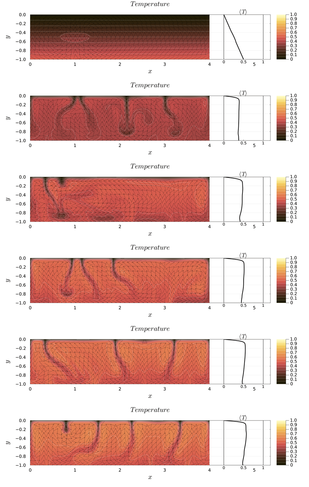
Figure 1. Evolution of internally heated thermal convection. Heat generated uniformly throughout the domain is transported toward the cold surface by convection, producing broad upwellings and narrow downwellings. The figure shows the temperature field, velocity vectors, and the horizontally averaged temperature profile during the simulation.
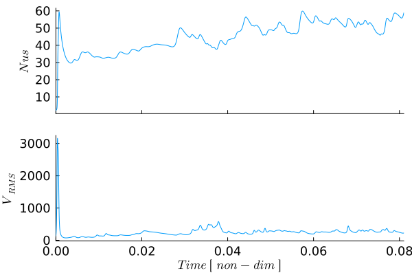
Figure 2. Evolution of the Nusselt number and root-mean-square velocity. These diagnostic quantities illustrate the transition from the initial conductive state toward vigorous convection and the subsequent approach to a statistically steady convective regime.
The following helper function generates the main visualization used throughout the example. It combines the temperature field, velocity vectors, and the horizontally averaged temperature profile into a single figure.
# ======================================================================= #
# Helper function ======================================================= #
# ======================================================================= #
function PlotFieldProfile(Pl,M,D,x,y,Tmean)
    # ---------------------------------------------------------------------------
    # Combined temperature field and mean-temperature profile
    # ---------------------------------------------------------------------------
    p = nothing

    # Width of the physical model domain
    Lx  =   M.xmax - M.xmin

    # Geometry of the profile strip
    profile_gap     =   0.08Lx       # Gap between field and profile
    profile_width   =   0.22Lx       # Width assigned to the profile

    xprofile_min    =   M.xmax + profile_gap
    xprofile_max    =   xprofile_min + profile_width

    # # Mean-temperature profile at the current time step
    # Tmean           =   meanT[it, :]

    # Map <T> = 0...1 onto the profile strip
    xprofile        =   xprofile_min .+ profile_width .* Tmean

    # Full horizontal extent of the combined figure
    xmax_plot       =   xprofile_max + 0.04Lx

    p = plot(
        size            = (1900, 500),
        dpi             = 300,
        guidefontsize   = 28,
        tickfontsize    = 18,
        titlefontsize   = 28,
        legend          = false,
        framestyle      = :box,
        left_margin     = 20mm,
        right_margin    = 10mm,
        bottom_margin   = 15mm,
        top_margin      = 8mm,
    )

    # ---------------------------------------------------------------------------
    # Temperature field
    # ---------------------------------------------------------------------------

    heatmap!(
        p,
        x.c,
        y.c,
        D.T',
        xlabel       = L"x",
        ylabel       = L"y",
        title        = L"Temperature",
        color        = cgrad(:lajolla),
        colorbar     = true,
        aspect_ratio = :equal,
        clims        = (0,1),
        xlims        = (M.xmin, xmax_plot),
        ylims        = (M.ymin, M.ymax),
    )

    contour!(
        p,
        x.c,
        y.c,
        D.T',
        linewidth = 1,
        color     = "white",
        alpha     = 0.5,
    )

    quiver!(
        p,
        x.c2d[1:Pl.qinc:end, 1:Pl.qinc:end],
        y.c2d[1:Pl.qinc:end, 1:Pl.qinc:end],
        quiver = (
            D.vxc[1:Pl.qinc:end, 1:Pl.qinc:end] .* Pl.qsc,
            D.vyc[1:Pl.qinc:end, 1:Pl.qinc:end] .* Pl.qsc,
        ),
        linewidth = 1,
        linealpha = 0.5,
        color     = "black",
    )

    # ---------------------------------------------------------------------------
    # Mean-temperature profile
    # ---------------------------------------------------------------------------

    # White background for the profile strip
    plot!(
        p,
        Shape(
            [xprofile_min, xprofile_max, xprofile_max, xprofile_min],
            [M.ymin, M.ymin, M.ymax, M.ymax],
        ),
        fillcolor   = :white,
        fillalpha   = 1.0,
        linecolor   = :black,
        linewidth   = 1.5,
    )

    # Optional horizontal reference lines
    for ytick in range(M.ymin, M.ymax, length=6)
        plot!(
            p,
            [xprofile_min, xprofile_max],
            [ytick, ytick],
            color     = :gray,
            alpha     = 0.25,
            linewidth = 0.8,
        )
    end

    # Mean-temperature profile
    plot!(
        p,
        xprofile,
        y.ce,
        color     = :black,
        linewidth = 4,
    )

    # Separator between field and profile
    vline!(
        p,
        [xprofile_min],
        color     = :black,
        linewidth = 1.5,
    )

    # Profile title
    annotate!(
        p,
        (
            0.5 * (xprofile_min + xprofile_max),
            M.ymax + 0.055 * (M.ymax - M.ymin),
            text(L"\langle T\rangle", 24, :center),
        ),
    )

    # Profile-axis labels: 0, 0.5, 1
    for (Ttick, label) in zip((0.0, 0.5, 1.0), ("0", "0.5", "1"))
        xtick = xprofile_min + profile_width * Ttick

        # Small tick mark
        plot!(
            p,
            [xtick, xtick],
            [M.ymin, M.ymin + 0.018 * (M.ymax - M.ymin)],
            color     = :black,
            linewidth = 1.2,
        )

        # Tick label
        annotate!(
            p,
            (
                xtick,
                M.ymin - 0.055 * (M.ymax - M.ymin),
                text(label, 16, :center),
            ),
        )
    end
    return p
end
# ======================================================================= #