RTI - Growth Rate Benchmark
This script benchmarks the growth rate of a Rayleigh-Taylor instability, following Gerya (2019). The benchmark is based on the analytical solution by Ramberg (1968) and is used to evaluate the accuracy of the velocity field in a purely gravity-driven flow.
The script calculates the diapiric growth rate at the tip of the perturbation for different perturbation amplitudes ($\delta A$), wavelengths ($\lambda$), and viscosity ratios ($\eta_r$). The numerical solution is plotted alongside the analytical one, which is arbitrarily scaled by certain constants for visualization purposes, following Gerya (2009).
The amplitude of the cosine perturbation is defined as:
\[\begin{equation} \delta A = \cos\left( 2\pi \frac{x_m - L/2}{\lambda} \right), \end{equation}\]
where $x_m$ is the x-coordinate of the marker, and $L$ is the length of the model domain. The perturbation is applied to the tracers by adding the perturbation amplitude to the y-coordinate of an initially equally distributed or randomly perturbed tracer field.
Using a bilinear interpolation scheme to map tracer properties onto the regular numerical grid, one can test how accurately the Stokes solver reproduces the analytical growth rate of the diapiric instability. However, care must be taken when defining the initial tracer positions or when averaging tracer properties onto the grid to avoid numerical artifacts.
Let's load the required modules first.
using Plots
using ExtendableSparse
using GeoModBox
using GeoModBox.InitialCondition, GeoModBox.MomentumEquation.TwoD
using GeoModBox.AdvectionEquation.TwoD
using GeoModBox.Tracers.TwoD
using Base.Threads
using Printf, LinearAlgebra
using TimerOutputs
function UpdateRheo(D,ρ,η,avg)
# Density --- artihmetic averaging ---
@. D.ρ = ρ[1]*(1.0 - D.p) + ρ[2]*D.p
D.ρe[2:end-1,2:end-1] .= D.ρ
D.ρe[1,:] .= D.ρe[2,:]
D.ρe[end,:] .= D.ρe[end-1,:]
D.ρe[:,1] .= D.ρe[:,2]
D.ρe[:,end] .= D.ρe[:,end-1]
# Viscosity - Centroids and vertices ---
if avg == :arith
@. D.ηc = (1.0 - D.p) * η[1] + D.p * η[2]
elseif avg == :harm
@. D.ηc = 1.0 / ( (1.0 - D.p) / η[1] + D.p / η[2] )
elseif avg == :geom
@. D.ηc = η[1]^(1.0 - D.p) * η[2]^D.p
else
error("Unknown viscosity averaging: $(avg)")
end
# --- Extended Centroids-
D.ηce[2:end-1,2:end-1] .= D.ηc
D.ηce[1,:] .= D.ηce[2,:]
D.ηce[end,:] .= D.ηce[end-1,:]
D.ηce[:,1] .= D.ηce[:,2]
D.ηce[:,end] .= D.ηce[:,end-1]
# --- Vertices -
if avg == :arith
@. D.ηv =
0.25*(
D.ηce[1:end-1,1:end-1] +
D.ηce[2:end ,1:end-1] +
D.ηce[1:end-1,2:end ] +
D.ηce[2:end ,2:end ]
)
elseif avg == :harm
@. D.ηv =
4.0/(
1/D.ηce[1:end-1,1:end-1] +
1/D.ηce[2:end ,1:end-1] +
1/D.ηce[1:end-1,2:end ] +
1/D.ηce[2:end ,2:end ]
)
elseif avg == :geom
@. D.ηv =
exp(0.25*(
log(D.ηce[1:end-1,1:end-1]) +
log(D.ηce[2:end ,1:end-1]) +
log(D.ηce[1:end-1,2:end ]) +
log(D.ηce[2:end ,2:end ])
))
else
error("Unknown viscosity averaging: $(avg)")
end
return D
endIn the following some parameters regarding the visualization can be edited.
to              = TimerOutput()
@timeit to "Ini" begin
plot_fields     =:no
save_fig        = 1
Pl  =   (
    qinc    =   5,
    qsc     =   100*(60*60*24*365.25)*5e1,
)
The parameters for an initial cosinusoidal tracer perturbation are defined for a two-layer model. For benchmarking purposes, a range of wavelengths is specified. One can define, if the density is interpolated from the tracers to the centroids or the vertices.
# How to update the numerical nodes from the marker ---
#   1) Phase ratio (:PhaseRatio), or
#   2) Direct bilinear interpolation of marker properties to the grid
#      (:MarkerInterpolation)
MaterialInterpolation   =   :MarkerInterpolation
# Define the averaging scheme used for both material-transfer methods:
#   1) Arithmetic   (:arith)
#   2) Geometric    (:geom)
#   3) Harmonic     (:harm)
avg                     =   :arith

MaterialInterpolation ∈ (:PhaseRatio, :MarkerInterpolation) ||
    error("Unknown material interpolation method: $MaterialInterpolation")
avg ∈ (:arith, :geom, :harm) ||
    error("Unknown averaging scheme: $avg")
# Although both strategies employ bilinear interpolation from the
# markers to the numerical grid, they differ in the quantity that is
# interpolated. The phase-ratio approach first interpolates the
# material phase and subsequently reconstructs the material
# properties using a mixing law, whereas the direct interpolation
# approach transfers the material properties themselves. Since
# viscosity is a nonlinear material property, the two approaches
# generally produce different numerical solutions.
# ------------------------------------------------------------------- #
# Define Initial Condition ========================================== #
# Density Averaging ---
#   centroids or vertices
# ρavg        =   :vertices
# Initial Marker distribution ---
Ini         =   (p=:RTI,)
nm          =   5
# Perturbation wavelength [ m ]
λᵣ          =   [3 4 5 6 8 9 10 12 14]*1e3
# ------------------------------------------------------------------- #
The physical parameters are now defined, including the range of viscosity ratios between the two layers.
# Physics =========================================================== #
g           =   9.81                    #   Gravitational acceleration [ m/s^2 ]
# Lower layer ---
ρ₁          =   2900.0                  #   Density composition 1 [ kg/m^3 ]
η₁          =   1e19                    #   Viscosity composition 1 [ Pa s]
# Upper layer ---
ρ₀          =   3000.0                  #   Density composition 0 [ kg/m^3 ]
# ---
ρ           =   [ρ₀,ρ₁]                 #   Density for phases
ηᵣ          =   [1e-6 1 10 100 500]     #   Viscosity ratio
phase       =   [0,1]
# Script notation:
#   phase 0: upper layer  (corresponds to η₁, ρ₁, h₁ in Gerya)
#   phase 1: lower layer  (corresponds to η₂, ρ₂, h₂ in Gerya)
# ------------------------------------------------------------------- #
In the following, the parameters for the analytical solution are initialized, some scaling parameters (b1 and b2) for the visualization, and the divisional factor for the perturbation wavelength (delfac)
# Plotting factors following Gerya (2019) --------------------------- #
b1          =   [0.5 1 5 50 250]
b2          =   [0.2 0.15 0.1 0.05 0]
# Divisional factor of the amplitude following Gerya (2019) --------- #
delfac      =   [15 150 1500]
ms          =   zeros(3)
ms          =   [8,6,4,2]
mc          =   ["black","red","yellow","green"]
# Analytical Solution ----------------------------------------------- #
λₐ          =   collect(LinRange(0.5,18,51)).*1e3        # [ m ]
ϕ₁          =   zeros(length(λₐ))
ϕ₂          =   copy(ϕ₁)
c11         =   copy(ϕ₁)
d12         =   copy(ϕ₁)
i21         =   copy(ϕ₁)
j22         =   copy(ϕ₁)
# Arrays ---
PP  =   (
    ϕ       =   [0.0],
    K       =   [0.0],
    Q       =   [0.0],
    ϕₐ      =   zeros(length(λₐ)),
    Kₐ      =   zeros(length(λₐ),length(ηᵣ)),
)
# ------------------------------------------------------------------- #
# Plot Settings ===================================================== #
q   =   plot()
# ------------------------------------------------------------------- #
Define the geometry of the model domain.
# Geometry ========================================================== #
M       =   Geometry(
    ymin    =   -3.0e3,     # [ m ]
    ymax    =   0.0,
    xmin    =   0.0,
)
# ------------------------------------------------------------------- #
end
If multiple perturbation amplitudes are specified, a loop is initiated over them. For each amplitude, a nested loop iterates over different viscosity contrasts. Within that loop the viscosity for the upper layer is calculated.
@timeit to "δA Loop" begin
for k in eachindex(delfac)
    @printf("δA = %g\n",delfac[k])
    @timeit to "ηr Loop" begin
    for i in eachindex(ηᵣ)
        # Physics =================================================== #
        # 0 - upper layer; 1 - lower layer
        η₀      =   η₁*ηᵣ[i]        #   Viscosity composition 0 [ Pa s ]
        η       =   [η₀,η₁]         #   Viscosity for phases
        @printf("   η₀ = %g\n",η₀)
        # ----------------------------------------------------------- #
The variables required for the analytical solution are calculated for each model configuration.
        # Analytical Solution ======================================= #
        @. ϕ₁      =   (2*π*((M.ymax-M.ymin)/2))/λₐ
        @. ϕ₂      =   (2*π*((M.ymax-M.ymin)/2))/λₐ
        @. c11     =   (η₀*2*ϕ₁^2)/
                        (η₁*(cosh(2*ϕ₁) - 1 - 2*ϕ₁^2)) -
                        (2*ϕ₂^2)/
                        (cosh(2*ϕ₂) - 1 - 2*ϕ₂^2)
        @. d12     =   (η₀*(sinh(2*ϕ₁) - 2*ϕ₁))/
                        (η₁*(cosh(2*ϕ₁) - 1 - 2*ϕ₁^2)) +
                        (sinh(2*ϕ₂) - 2*ϕ₂)/
                        (cosh(2*ϕ₂) - 1 - 2*ϕ₂^2)
        @. i21     =   (η₀*ϕ₂*(sinh(2*ϕ₁) + 2*ϕ₁))/
                        (η₁*(cosh(2*ϕ₁) - 1 - 2*ϕ₁^2)) +
                        (ϕ₂*(sinh(2*ϕ₂) + 2*ϕ₂))/
                        (cosh(2*ϕ₂) - 1 - 2*ϕ₂^2)
        @. j22     =   (η₀*2*ϕ₁^2*ϕ₂)/
                        (η₁*(cosh(2*ϕ₁) - 1 - 2*ϕ₁^2)) -
                        (2*ϕ₂^3)/
                        (cosh(2*ϕ₂) - 1 - 2*ϕ₂^2)

        PP.Kₐ[:, i] .= abs.(d12 ./ (c11 .* j22 .- d12 .* i21))
        @. PP.ϕₐ        =   ϕ₁
        # ----------------------------------------------------------- #
Because the analytical solution is independent of perturbation amplitude, the loop over different amplitudes is performed separately. Within that loop, both the model domain and perturbation amplitude are defined for each configuration.
        @timeit to "λ Loop" begin
        for j in eachindex(λᵣ)
            @timeit to "Ini2" begin
            # Perturbation properties ---
            λ           =   λᵣ[j]                           #   [ m ]
            δA          =   -(M.ymax-M.ymin)/2/delfac[k]    #   Amplitude [ m ]
            @printf("δA = %g\n",δA)
            # ---
            # Horizontal model width following Gerya (2019): L = 2λ
            M.xmax      =   M.xmin + 2.0 * λ
            @printf("       xmax: %g \n",M.xmax)
            @printf("       λ = %g\n",λ)
            # ------------------------------------------------------- #
            # Grid ================================================== #
            NC  =   (
                x   =   50,#*ar,
                y   =   50,
            )
            NV  =   (
                x   =   NC.x + 1,
                y   =   NC.y + 1,
            )
            Δ       =   GridSpacing(
                x   =   (M.xmax - M.xmin)/NC.x,
                y   =   (M.ymax - M.ymin)/NC.y,
            )
            x       =   (
                c   =   LinRange(M.xmin+Δ.x/2,M.xmax-Δ.x/2,NC.x),
                ce  =   LinRange(M.xmin - Δ.x/2.0, M.xmax + Δ.x/2.0, NC.x+2),
                v   =   LinRange(M.xmin,M.xmax,NV.x),
            )
            y       =   (
                c   =   LinRange(M.ymin+Δ.y/2,M.ymax-Δ.y/2,NC.y),
                ce  =   LinRange(M.ymin - Δ.y/2.0, M.ymax + Δ.y/2.0, NC.y+2),
                v   =   LinRange(M.ymin,M.ymax,NV.y),
            )
            x1      =   (
                c2d     =   x.c .+ 0*y.c',
                v2d     =   x.v .+ 0*y.v',
                vx2d    =   x.v .+ 0*y.ce',
                vy2d    =   x.ce .+ 0*y.v',
            )
            x   =   merge(x,x1)
            y1      =   (
                c2d     =   0*x.c .+ y.c',
                v2d     =   0*x.v .+ y.v',
                vx2d    =   0*x.v .+ y.ce',
                vy2d    =   0*x.ce .+ y.v',
            )
            y   =   merge(y,y1)
            # ------------------------------------------------------- #
Let's initialize all the required data array in the following.
            # Allocation ============================================ #
            D       =   (
                ρ       =   zeros(Float64,(NC...)),
                ρe      =   zeros(Float64,(NC.x+2,NC.y+2)),
                cp      =   zeros(Float64,(NC...)),
                vx      =   zeros(Float64,(NV.x,NV.y+1)),
                vy      =   zeros(Float64,(NV.x+1,NV.y)),
                Pt      =   zeros(Float64,(NC...)),
                vxc     =   zeros(Float64,(NC...)),
                vyc     =   zeros(Float64,(NC...)),
                vc      =   zeros(Float64,(NC...)),
                wt      =   zeros(Float64,(NC.x,NC.y)),
                wte     =   zeros(Float64,(NC.x+2,NC.y+2)),
                wtv     =   zeros(Float64,(NV.x,NV.y)),
                ηc      =   zeros(Float64,NC...),
                ηce     =   zeros(Float64,(NC.x+2,NC.y+2)),
                ηv      =   zeros(Float64,NV...),
                p       =   zeros(Float64,NC...),
                p_ex    =   zeros(Float64,(NC.x+2,NC.y+2)),
            )
            # ------------------------------------------------------- #
            # Needed for the defect correction solution ---
            divV        =   zeros(Float64,NC...)
            ε           =   (
                xx      =   zeros(Float64,NC...),
                yy      =   zeros(Float64,NC...),
                xy      =   zeros(Float64,NV...),
            )
            τ           =   (
                xx      =   zeros(Float64,NC...),
                yy      =   zeros(Float64,NC...),
                xy      =   zeros(Float64,NV...),
            )
            # ------------------------------------------------------- #
Also one needs to set the velocity boudnary conditions.
            # Boundary Conditions =================================== #
            VBC     =   (
                type    =   (E=:freeslip,W=:freeslip,S=:noslip,N=:noslip),
                val     =   (E=zeros(NV.y),W=zeros(NV.y),S=zeros(NV.x),N=zeros(NV.x),
                                vyS=0.0,vyN=0.0,vxW=0.0,vxE=0.0),
            )
            # ------------------------------------------------------- #
To setup the perturbation, the markers are initialized in the following.
            # Tracer Advection ====================================== #
            @timeit to "Tracer Ini" begin
            nmx,nmy     =   nm,nm
            noise       =   0
            nmark       =   nmx*nmy*NC.x*NC.y
            Aparam      =   :phase
            MPC         =   (
                c       =   zeros(Float64,(NC.x,NC.y)),
                v       =   zeros(Float64,(NV.x,NV.y)),
                th      =   zeros(Float64,(nthreads(),NC.x,NC.y)),
                thv     =   zeros(Float64,(nthreads(),NV.x,NV.y)),
            )
            MAVG        = (
                PC_th   =   [similar(D.wte) for _ = 1:nthreads()],  # per thread
                PV_th   =   [similar(D.wtv) for _ = 1:nthreads()],   # per thread
                wte_th  =   [similar(D.wte) for _ = 1:nthreads()],  # per thread
                wtv_th  =   [similar(D.wtv) for _ = 1:nthreads()],  # per thread
            )
            # Initialize Tracer Position ---
            Ma      =   IniTracer2D(Aparam,nmx,nmy,Δ,M,NC,noise,Ini.p,phase;λ,δA)
            # Count tracer per cell ---
            CountMPC(Ma,nmark,MPC,M,x,y,Δ,NC,NV)
            if MaterialInterpolation == :PhaseRatio
                # Phase ---
                Markers2Cells(Ma,nmark,MAVG.PC_th,D.p_ex,MAVG.wte_th,D.wte,x,y,Δ,Aparam,phase)
                D.p     .=  D.p_ex[2:end-1,2:end-1]
                UpdateRheo(D,ρ,η,avg)
            elseif MaterialInterpolation == :MarkerInterpolation
                # Interpolate from markers to cell ---
                Markers2Cells(Ma,nmark,MAVG.PC_th,D.p_ex,MAVG.wte_th,D.wte,x,y,Δ,Aparam,phase)
                D.p     .=  D.p_ex[2:end-1,2:end-1]
                Markers2Cells(Ma,nmark,MAVG.PC_th,D.ρe,MAVG.wte_th,D.wte,x,y,Δ,Aparam,ρ)
                D.ρ     .=   D.ρe[2:end-1,2:end-1]
                Markers2Cells(Ma,nmark,MAVG.PC_th,D.ηce,MAVG.wte_th,D.wte,x,y,Δ,Aparam,η;avgm=avg)
                D.ηc    .=   D.ηce[2:end-1,2:end-1]
                Markers2Vertices(Ma,nmark,MAVG.PV_th,D.ηv,MAVG.wtv_th,D.wtv,x,y,Δ,Aparam,η;avgm=avg)
            else
                error("Unknown material interpolation method: $MaterialInterpolation")
            end
            end
            # ------------------------------------------------------- #
The parameters for solving the linear system using the defect correction method are now defined.
            # System of Equations =================================== #
            # Iterations
            niter       =   50
            ϵ           =   1e-10
            # Numbering, without ghost nodes! ---
            off    = [  NV.x*NC.y,                          # vx
                        NV.x*NC.y + NC.x*NV.y,              # vy
                        NV.x*NC.y + NC.x*NV.y + NC.x*NC.y]  # Pt

            Num    =    (
                Vx  =   reshape(1:NV.x*NC.y, NV.x, NC.y),
                Vy  =   reshape(off[1]+1:off[1]+NC.x*NV.y, NC.x, NV.y),
                Pt  =   reshape(off[2]+1:off[2]+NC.x*NC.y,NC...),
                        )
            δx      =   zeros(maximum(Num.Pt))
            F       =   zeros(maximum(Num.Pt))
            # Residuals ---
            Fm     =    (
                x       =   zeros(Float64,NV.x, NC.y),
                y       =   zeros(Float64,NC.x, NV.y)
            )
            FPt     =   zeros(Float64,NC...)
            # ------------------------------------------------------- #
            end
The momentum and mass conservation equations are now solved.
            # Momentum Equation ===
            D.vx    .=  0.0
            D.vy    .=  0.0
            D.Pt    .=  1.0
            @timeit to "Solution Iteration" begin
            # Assemble Coefficients ========================================= #
            @timeit to "Assembly" begin
            K       =   Assembly(NC, NV, Δ, D.ηc, D.ηv, VBC, Num)
            Kfac    =   lu(K.cscmatrix)
            end
            for iter=1:niter
                # Initial Residual -------------------------------------- #
                @timeit to "Residual" begin
                Residuals2D!(D,VBC,ε,τ,divV,Δ,D.ηc,D.ηv,g,Fm,FPt)
                F[Num.Vx]   .=   Fm.x
                F[Num.Vy]   .=   Fm.y
                F[Num.Pt]   .=   FPt
                @printf("||R|| = %1.4e\n", norm(F)/length(F))
                norm(F)/length(F) < ϵ ? break : nothing
                end
                # ------------------------------------------------------- #
                # Solution of the linear system ========================= #
                @timeit to "Solution" begin
                δx      =   - (Kfac \ F)
                end
                # ------------------------------------------------------- #
                # Update Unknown Variables ============================== #
                D.vx[:,2:end-1]     .+=  δx[Num.Vx]
                D.vy[2:end-1,:]     .+=  δx[Num.Vy]
                D.Pt                .+=  δx[Num.Pt]
            end
            end
            # ------------------------------------------------------- #
For visualization purposes, the centroid velocities are computed.
            # Get the velocity on the centroids ---
            # Just for visualization purposes
            for i = 1:NC.x
                for j = 1:NC.y
                    D.vxc[i,j]  = (D.vx[i,j+1] + D.vx[i+1,j+1])/2
                    D.vyc[i,j]  = (D.vy[i+1,j] + D.vy[i+1,j+1])/2
                end
            end
            @. D.vc        = sqrt(D.vxc^2 + D.vyc^2)
In the following, one defines the parameters to calculate the rising velocity at the tip of the perturbation in the center of the model domain. The vertical velocity at the perturbation tip is calculated using bilinear interpolation from surrounding velocity grid points.
            @timeit to "Calc GR" begin
            # Calculate diapir growth rate ---
            xwave       =   (M.xmax-M.xmin)/2
            ywave       =   (M.ymax-M.ymin)/2 + δA

            xn          =   Int64(floor((xwave+Δ.x/2)/Δ.x))
            yn          =   Int64(floor(((M.ymax-M.ymin)-ywave)/Δ.y)) + 1

            dx          =   (xwave+Δ.x/2)/Δ.x - xn
            dy          =   abs(((M.ymax-M.ymin)-ywave)/Δ.y - yn)

            wvy     =   (1.0-dx)*(1.0-dy) * D.vy[xn+1,yn] +
                            dx*(1.0-dy) * D.vy[xn+2,yn] +
                            (1.0-dx)*dy * D.vy[xn+1,yn+1] +
                            dx*dy * D.vy[xn+2,yn+1]

            PP.Q[1] =   (ρ₀-ρ₁)*(M.ymax-M.ymin)/2.0*g/2.0/η₁
            PP.K[1] =   abs(wvy)/abs(δA)/PP.Q[1]
            PP.ϕ[1] =   2*π*(M.ymax-M.ymin)/2/λ
            end
If wanted, the density, tracer, and viscosity fields are plotted. To verify the position of the perturbation tip used in velocity interpolation, the tip (black circle) and surrounding vertical velocity grid points (red circles) are plotted on the tracer field. The plot is zoomed in for better visualization.
            if plot_fields==:yes
                p = heatmap(x.c./1e3,y.c./1e3,D.ρ',color=:inferno,
                            xlabel="x[km]",ylabel="y[km]",colorbar=true,
                            title="ρ",
                            aspect_ratio=:equal,xlims=(M.xmin/1e3, M.xmax/1e3),
                            ylims=(M.ymin/1e3, M.ymax/1e3),
                            layout=(3,1),subplot=1)
                quiver!(p,x.c2d[1:Pl.qinc:end,1:Pl.qinc:end]./1e3,
                    y.c2d[1:Pl.qinc:end,1:Pl.qinc:end]./1e3,
                    quiver=(D.vxc[1:Pl.qinc:end,1:Pl.qinc:end].*Pl.qsc,
                            D.vyc[1:Pl.qinc:end,1:Pl.qinc:end].*Pl.qsc),
                    la=0.5,color="white",layout=(3,1),subplot=1)
                scatter!(p,Ma.x[1:end]./1e3,Ma.y[1:end]./1e3,
                    ms=3,ma=0.5,mc=Ma.phase[1:end],markerstrokewidth=0.0,
                    xlabel="x[km]",ylabel="y[km]",colorbar=true,
                    title="tracers",label="",
                    xlims=(xwave/1e3-Δ.x/1e3*1.1, xwave/1e3+Δ.x/1e3*1.1),
                    ylims=(-ywave/1e3-Δ.y/1e3*1.1, -ywave/1e3+Δ.y/1e3*1.1),
                    layout=(3,1),subplot=3)
                heatmap!(p,x.c./1e3,y.c./1e3,log10.(abs.(D.ηc)'),
                            color=reverse(cgrad(:roma)),
                            xlabel="x[km]",ylabel="y[km]",title="η_c",
                            clims=(15,27),
                            aspect_ratio=:equal,xlims=(M.xmin/1e3, M.xmax/1e3),
                            ylims=(M.ymin/1e3, M.ymax/1e3),colorbar=true,
                            layout=(2,1),subplot=2)
                scatter!(p,(xwave/1.0e3,-ywave/1.0e3),
                        markersize=3,label="",color=:black,
                        layout=(3,1),subplot=3)
                scatter!(p,(x1.vy2d[xn+1,yn]/1e3,y1.vy2d[xn+1,yn]/1e3),
                        markersize=3,label="",color=:blue,
                        layout=(3,1),subplot=3)
                scatter!(p,(x1.vy2d[xn+2,yn]/1e3,y1.vy2d[xn+2,yn]/1e3),
                        markersize=3,label="",color=:blue,
                        layout=(3,1),subplot=3)
                scatter!(p,(x1.vy2d[xn+1,yn+1]/1e3,y1.vy2d[xn+1,yn+1]/1e3),
                        markersize=3,label="",color=:blue,
                        layout=(3,1),subplot=3)
                scatter!(p,(x1.vy2d[xn+2,yn+1]/1e3,y1.vy2d[xn+2,yn+1]/1e3),
                        markersize=3,label="",color=:blue,
                        layout=(3,1),subplot=3)
                display(p)
            end
            scatter!(q,(PP.ϕ[1],b1[i]*PP.K[1] + b2[i]),
                ms=ms[k],markershape=:circle,label="",
                color=mc[k])
        end # Loop λ - j
        end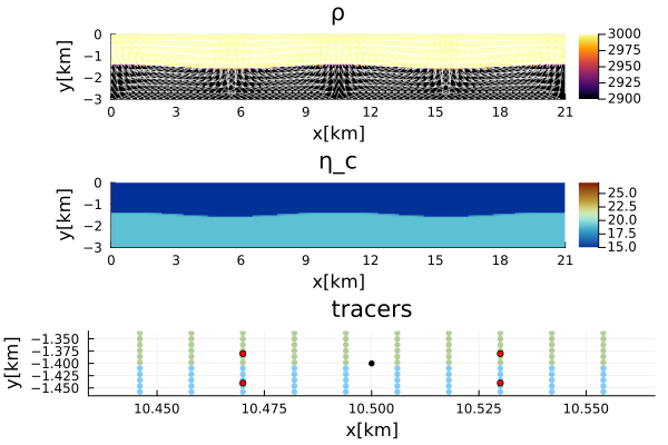
Figure 1. Example of a RTI model. Top: Centroid velocity arrows on top of the density field. Middle: Centroid viscosity. Bottom: Zoom of the tracer field on the tip of the perturbation at the center of the model domain. The black tracer marks the tip, and the red tracer mark the vertical velocity nodes from which the vertical velocity is interpolated onto the tip. This example uses a perturbation of $A = h_{1}/15$ and a wavelength of 12 km. The model includes 50 centroids in the vertical direction. The number of horizontal centroids is chosen such that the resolution remains consistent in both the horizontal and vertical directions for all benchmark models.
Finally, the rising velocity is plotted over the analytical solution for the given range of viscosity contrasts.
        if k == 1
            plot!(q,PP.ϕₐ,b1[i].*PP.Kₐ[:,i] .+ b2[i],
                        xlabel="ϕ₁ = 2πh₁/λ",
                        ylabel="b₁K + b₂",
                        title="",
                        xlims=(0.5,4),ylims=(0.05,0.5),
                        label=string("ηᵣ = ", ηᵣ[i]))
        end
    end # Loop ηᵣ - i
    end
end # Loop delfac - k
end
The final figure is stored in the given directory.
if save_fig == 1
    savefig(q,string("./examples/StokesEquation/2D/Results/RTI_Growth_Rate_nmx_",nm,
                        "_nmy_",nm,"_",MaterialInterpolation,"_",avg,".png"))
else
    display(q)
end
display(to)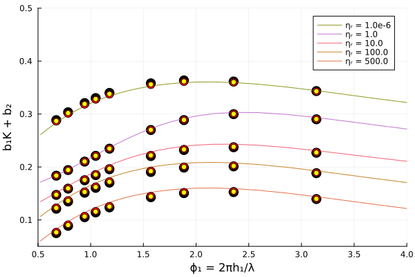
Figure 2. RTI Growth Rate. Growth rate of an initial cosinusoidal perturbation in a two-layer system across various wavelengths $\lambda$. The growth rate is arbitrarily scaled using $b_1$ and $b_2$ for visualization, following the approach of Gerya (2019). The lines are the analytical solutions for different viscosity ratios $\eta_r$ and the markers show the corresponding numerical results for models with decreasing amplitudes (black - 100 m, red - 10 m, yellow - 1 m). The rising velocity is numerically calculated following the approach shown in Figure 1.
Resolution Test
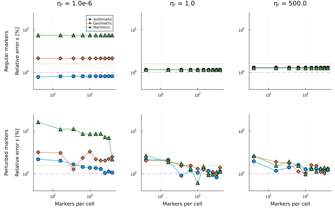
Figure 3. RTI Resolution Test. Relative error ε in [%] for the RTI growth rate using a fixed layer thickness (1500 km), a fixed wavelength $\lambda = 4000 \text{ km}$, a fixed perturbation amplitudes $\left(\delta{A} = 1 \textrm{m} \right)$, and a fixed horizontal and vertical grid resolutions $\left(nc_x,nc_y\right)$ for an increasing number of markers per cell and different viscosity ratios $\eta_r$ including regular distributed (top row) or randomly distributed (bottom row) initial marker positions (before assigning the layer phases). The viscosity is interpolate from the tracers to the centroids and the vertices using an either arithmetic (circle), geometric (diamond), or harmonic (triangle) mean.
The summary figure compares the relative error of the numerical growth rate for the three viscosity averaging schemes using both regular and randomly perturbed marker distributions. Each panel shows the error as a function of the number of markers per cell for a fixed viscosity ratio.
For moderate viscosity contrasts ($\eta_r = 1$ and $\eta_r = 500$), all three averaging schemes produce comparable results, and increasing the marker density only slightly improves the accuracy. In contrast, for the extreme viscosity contrast ($\eta_r = 10^{-6}$), the choice of averaging scheme becomes critical. Arithmetic averaging consistently yields the smallest errors and is largely insensitive to the marker distribution, whereas geometric averaging introduces noticeably larger errors. Harmonic averaging performs poorly for this benchmark and remains inaccurate even for large numbers of markers.
The comparison demonstrates that, for marker-in-cell simulations with strong viscosity contrasts, the choice of viscosity averaging scheme has a significantly greater influence on the numerical accuracy than the marker density itself. Increasing the number of markers cannot compensate for an unsuitable averaging scheme, while arithmetic averaging provides the most robust and accurate results for the Rayleigh-Taylor instability benchmark.
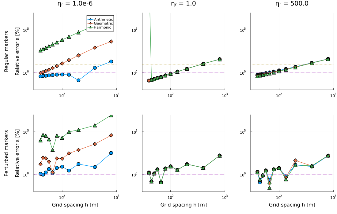
Figure 4. RTI Resolution Test. Relative error ε in [%] for the RTI growth rate using a fixed layer thickness (1500 km), a fixed wavelength $\lambda = 4000 \text{ km}$, a fixed perturbation amplitudes $\left(\delta{A} = 1 \textrm{m} \right)$, and a fixed number of markers per cell (5x5) for an increasing horizontal and vertical grid resolutions $\left(nc_x,nc_y\right)$ and different viscosity ratios $\eta_r$ including regular distributed (top row) or randomly distributed (bottom row) initial marker positions (before assigning the layer phases). The viscosity is interpolate from the tracers to the centroids and the vertices using an either arithmetic (circle), geometric (diamond), or harmonic (triangle) mean.
The grid-resolution test compares the relative error of the numerical RTI growth rate as the characteristic grid spacing is reduced while maintaining a constant number of markers per cell. For moderate viscosity ratios ($\eta_r=1$ and $\eta_r=500$), all three viscosity averaging schemes show comparable behaviour and generally approach the analytical solution with increasing grid resolution. For the extreme viscosity ratio $\eta_r=10^{-6}$, however, the averaging scheme has a much stronger influence than the grid spacing. Arithmetic averaging consistently produces the smallest errors, whereas geometric and particularly harmonic averaging introduce substantial systematic deviations that are not removed by grid refinement.
Random perturbations of the marker positions increase the scatter of the numerical error, especially at coarse resolution, but do not change the overall ranking of the averaging schemes. The results therefore demonstrate that increasing spatial resolution cannot compensate for an unsuitable treatment of viscosity across a sharp material interface. They also confirm that the choice between direct marker interpolation and phase-ratio-based reconstruction has only a secondary influence when the same averaging scheme is used.