Diffusion Equation (Backward Euler)
This example introduces the conservative finite-difference formulation for the transient two-dimensional diffusion equation using the general residual–matrix framework. Although the present problem is linear and converges in a single iteration, the defect-correction algorithm provides the foundation for solving nonlinear diffusion problems with temperature-dependent material properties. The focus lies on the
- application of the expanded temperature field and boundary conditions,
- set up of the coefficient matrix and residual vector,
- implementation of the analytical solution (
ExactFieldSolution.jl), and - application of the defect correction method.
The example calculates the numerical solution of a transient diffusion of an initial, Gaussian 2-D temperature distribution. The peak $T0$ of the Gaussian anomaly is located in the center of the model domain with a certain width $\sigma$. In this example, the thermal diffusivity is $K=10^{−6}$. Since ρ=cp=1, the thermal conductivity takes the same numerical value.
The accuracy of the numerical solution is checked with its analytical solution. The results are plotet for ever nout time step in a single figure.
First one needs to load the required packages:
using GeoModBox.HeatEquation.TwoD
using ExactFieldSolutions, LinearAlgebra, Plots, Printf
Now, one needs to define the geometry and the numerical parameters.
# Spatial domain
xlim = (min=-1/2, max=1/2)
ylim = (min=-1/2, max=1/2)
nc   = (x=100, y=100)
nv   = (x=nc.x+1, y=nc.y+1)
nc   = (x=nc.x+0, y=nc.y+0)
nv   = (x=nv.x+0, y=nv.y+0)
Δ    = (x=(xlim.max-xlim.min)/nc.x, y=(ylim.max-ylim.min)/nc.y)
x    = (c=LinRange(xlim.min+Δ.x/2, xlim.max-Δ.x/2, nc.x), v=LinRange(xlim.min, xlim.max, nv.x))
y    = (c=LinRange(ylim.min+Δ.y/2, ylim.max-Δ.y/2, nc.y), v=LinRange(ylim.min, ylim.max, nv.y))
Now, one needs to define the time parameters and parameters for the solution iteration.
# Time domain
nt   = 500
t    = 0.
nout = 10
# Iterations
niter = 10
ϵ     = 1e-10
In the following, all fields and parameter arrays are initialized.
# Primitive variables
T_ex  = zeros(nc.x+2, nc.y+2)
T_ex0 = zeros(nc.x+2, nc.y+2)
T     = zeros(nc...)
T0    = zeros(nc...)
Te    = zeros(nc...)
# Derived fields
∂T    = (∂x=zeros(nv.x, nc.x), ∂y=zeros(nc.x, nv.x),
            ∂x0=zeros(nv.x, nc.x), ∂y0=zeros(nc.x, nv.x))
q     = (x=zeros(nv.x, nc.x), y=zeros(nc.x, nv.x),
            x0=zeros(nv.x, nc.x), y0=zeros(nc.x, nv.x))
# Material parameters
ρ     = zeros(nc...)
Cp    = zeros(nc...)
Q     = zeros(nc...)
k     = (x=zeros(nv.x, nc.x), y=zeros(nc.x, nv.x))
# Residuals
R     = zeros(nc...)
The expanded temperature field includes one layer of ghost nodes surrounding the computational domain. These ghost nodes allow Dirichlet and Neumann boundary conditions to be incorporated while keeping the finite-difference stencil identical throughout the domain.
Here, the boundary conditions are defined, using a named tuple BC. The tuple contains the type (Dirichlet or Neumann) and the value of each boundary (North, East, South, West). Additionally, the array for the numbering of the equation is initialized.
# Boundary conditions
BC   = (
    type = (W=:Dirichlet, E=:Dirichlet, S=:Dirichlet, N=:Dirichlet),
    # type = (W=:Neumann, E=:Neumann, S=:Neumann, N=:Neumann),
    val  = (W=zeros(nc.y), E=zeros(nc.y), S=zeros(nc.x), N=zeros(nc.x)))
# Numbering
Num    = (T=reshape(1:nc.x*nc.y, nc.x, nc.y),)
As initial condition, the analytical solution for the time $t=0$ is choosen. Also, the values for the physical parameter are assigned. Here, all parameters are non-dimensional.
# Initial conditions
AnalyticalSolution2D!(T, x.c, y.c, t,(T0=1.0,K=1e-6,σ=0.1))
@. k.x = 1e-6
@. k.y = 1e-6
@. ρ   = 1.0
@. Cp  = 1.0
Δt = max(Δ...)^2/(maximum(k.x)/minimum(ρ)/minimum(Cp))/4.1
Although the Backward Euler method is unconditionally stable, the time step is chosen according to the explicit stability criterion. Using the same time step facilitates comparison with the explicit diffusion examples presented earlier.
Now, the time loop can start. Within the time loop, the time, the analytical solution and the value for the boundaries is calculated within the following.
# Time integration Loop
for it=1:nt
    @printf("Time step = %05d\n", it)
    t += Δt
    @. T0 = T
    # Exact solution on cell centroids
    AnalyticalSolution2D!(Te, x.c, y.c, t,(T0=1.0,K=1e-6,σ=0.1))
    # Exact solution on cell boundaries
    BoundaryConditions2D!(BC, x.c, y.c, t,(T0=1.0,K=1e-6,σ=0.1))
To enable a direct comparison with the analytical solution, the Dirichlet boundary conditions are updated at every time step using the analytical temperature field evaluated on the domain boundaries.
The temperature conservation equation is solved in the following using the defect correction method. Therefore, one first needs to determine the residual (ComputeResiduals2D!()) of the system of equations, assuming an initial guess. If the residual is small enough (ϵ), the solution iteration is stopped.
Note: The iteration is only necessary, if the system is non-linear. Here, the final solution is found after one iteration. Consequently, the residual becomes essentially zero after the first defect-correction step. The iteration loop is retained to demonstrate the general solution procedure used later for nonlinear diffusion and Stokes problems.
For more details on the defect correction method, please refer to the documentation.
# Iteration loop
    for iter=1:niter
        # Evaluate residual
        ComputeResiduals2D!(R, T, T_ex, T0, T_ex0, Q, ∂T, q, ρ, Cp, k, BC, Δ, Δt)
        @printf("||R|| = %1.4e\n", norm(R)/length(R))
        norm(R)/length(R) < ϵ ? break : nothing
        # Assemble linear system
        K  = AssembleMatrix2D(ρ, Cp, k, BC, Num, nc, Δ, Δt)
        # Solve for temperature correction: Cholesky factorisation
        Kc = cholesky(K.cscmatrix)
        # Solve for temperature correction: Back substitutions
        δT = -(Kc\R[:])
        # Update temperature
        @. T += δT[Num.T]
    end
Finally, the analytical and numerical solution and its error are plotted for each nout time step.
    # Visualisation
    if mod(it, nout)==0
        p1 = plot(aspect_ratio=1, xlims=(xlim...,), ylims=(ylim...,))
        p1 = heatmap!(x.c, y.c, Te', title="Analytics")
        p2 = plot(aspect_ratio=1, xlims=(xlim...,), ylims=(ylim...,))
        p2 = heatmap!(x.c, y.c, T', title="Numerics")
        p3 = plot(aspect_ratio=1, xlims=(xlim...,), ylims=(ylim...,))
        p3 = heatmap!(x.c, y.c, (abs.(T-Te))', title="Error")
        display(plot(p1, p2, p3, layout=(2,2)))
    end
end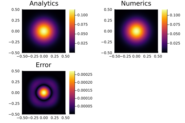
Figure 1. Final plot for the backward Euler solution using the defect correction method.